Artificial Intelligence
Recurrent Neural Networks (RNN): Deep Learning for Sequential Data
June 17, 2020
8 min read


Recurrent Neural Networks (RNN) are a class of Artificial Neural Networks that can process a sequence of inputs in deep learning and retain its state while processing the next sequence of inputs. Traditional neural networks will process an input and move onto the next one disregarding its sequence. Data such as time series have a sequential order that needs to be followed in order to understand. Traditional feed-forward networks cannot comprehend this as each input is assumed to be independent of each other whereas in a time series setting each input is dependent on the previous input.
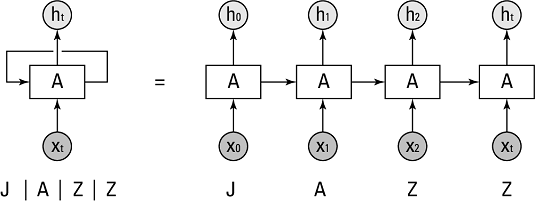
In Illustration 1 we see that the neural network (hidden state) A takes an xt and outputs a value ht. The loop shows how the information is being passed from one step to the next. The inputs are the individual letters of ‘JAZZ’ and each one is passed on to the network A in the same order it is written (i.e. sequentially).
Recurrent Neural Networks can be used for a number of ways such as:
An autoregressive model is when a value from data with a temporal dimension are regressed on previous values up to a certain point specified by the user. An RNN works the same way but the obvious difference in comparison is that the RNN looks at all the data (i.e. it does not require a specific time period to be specified by the user.)
Yt = β0 + β1yt-1 + Ɛt
The above AR model is an order 1 AR(1) model that takes the immediate preceding value to predict the next time period’s value (yt). As this is a linear model, it requires certain assumptions of linear regression to hold–especially due to the linearity assumption between the dependent and independent variables. In this case, Yt and yt-1 must have a linear relationship. In addition there are other checks such as autocorrelation that have to be checked to determine the adequate order to forecast Yt.
An RNN will not require linearity or model order checking. It can automatically check the whole dataset to try and predict the next sequence. As demonstrated in the image below, a neural network consists of 3 hidden layers with equal weights, biases and activation functions and made to predict the output.
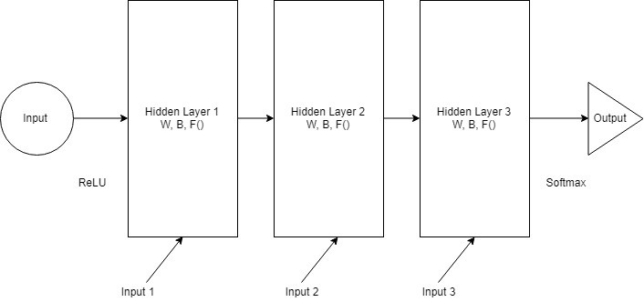
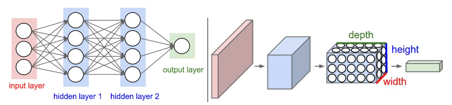
These hidden layers can then be merged to create a single recurrent hidden layer. A recurrent neuron now stores all the previous step input and merges that information with the current step input.
As more layers containing activation functions are added, the gradient of the loss function approaches zero. The gradient descent algorithm finds the global minimum of the cost function of the network. Shallow networks shouldn’t be affected by a too small gradient but as the network gets bigger with more hidden layers it can cause the gradient to be too small for model training.
Gradients of neural networks are found using the backpropagation algorithm whereby you find the derivatives of the network. Using the chain rule, derivatives of each layer are found by multiplying down the network. This is where the problem lies. Using an activation function like the sigmoid function, the gradient has a chance of decreasing as the number of hidden layers increase.
This issue can cause terrible results after compiling the model. The simple solution to this has been to use Long-Short Term Memory models with a ReLU activation function.

Long-Short Term Memory Networks are a special type of Recurrent Neural Networks that are capable of handling long term dependencies without being affected by an unstable gradient.
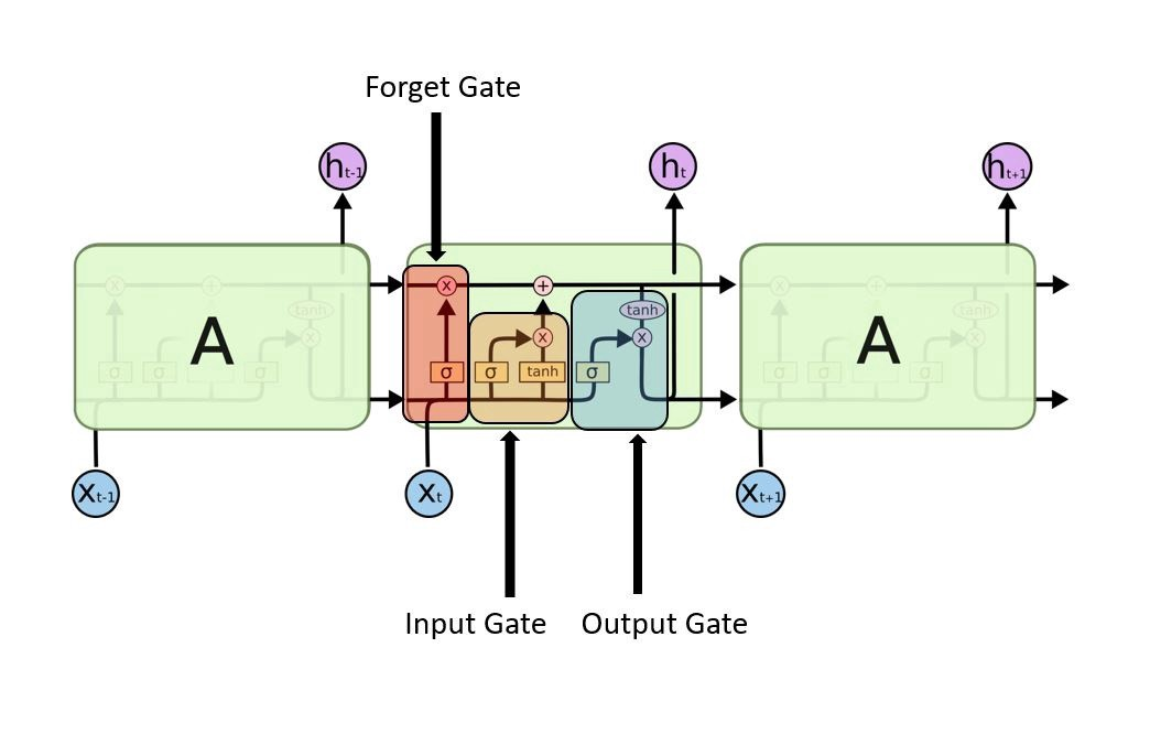
The above diagram is a typical RNN except that the repeating module contains extra layers that distinguishes itself from an RNN.
The differentiation here is the horizontal line called the ‘cell state’ that acts as a conveyor belt of information. The LSTM will remove or add information to the cell state by using the 3 gates as illustrated above. The gates are composed of a sigmoid function and a point-wise multiplication operation that outputs between 1 and 0 to describe how much of each component to let through the cell state. A value of 1 means to let all the information through while 0 means to completely disregard it.
The 3 gates are:
1) Input gate - This gate is used to discover which value will be used to modify the memory using the sigmoid function (by assigning a value between 0 and 1) followed by a tanh function which gives a weightage to the value between -1 to 1.
2) Forget gate - The forget gate decides which value to disregard using a sigmoid function by using the previous state (ht-1) and the input (xt) by assigning a value between 0 and 1 for each value in ct-1.
3) Output gate - The input of this block is used to decide the output by using a sigmoid function to assign a value between 0 and 1 followed by multiplying by a tanh function to decide its level of importance by assigning a value between -1 and 1.
## Libraries
import tensorflow as tf

model = tf.keras.models.Sequential()
Dense = tf.keras.layers.Dense
Dropout = tf.keras.layers.Dropout
LSTM = tf.keras.layers.LSTM
## Dataset
mnist_data = tf.keras.datasets.mnist
# mnist is a dataset of 28x28 images of handwritten digits and their labels with 60,000 rows of data
## Create train and test data
(x_train, y_train),(x_test, y_test) = mnist_data.load_data()

x_train = x_train/255.0 # Normalize training data features
x_test = x_test/255.0 # Normalize training data labels
#The images are 28x28 pixels of unassigned integers in the range of 0 to 255. The above #normalization code is not necessary and can still be passed on to compile. However, the #accuracy will be much worse of at around 20% best case scenario and loss at over 90%. The #training time will also increase.
model.add(LSTM(256, activation='relu', return_sequences=True))
model.add(Dropout(0.2))

model.add(LSTM(256, activation='relu'))
model.add(Dropout(0.1))

model.add(Dense(32, activation='relu'))
model.add(Dropout(0.2))

model.add(Dense(10, activation='softmax'))

optimizer = tf.keras.optimizers.Adam(lr=1e-4, decay=1e-6)
# Compile model
model.compile(
loss='sparse_categorical_crossentropy',
optimizer=optimizer,
metrics=['accuracy'],
)
# The specification of loss=’sparse_categorical_crossentropy’ is very important here as our targets are # integers and not one-hot encoded categories.
model.fit(x_train,
y_train,
epochs=4,
validation_data=(x_test, y_test))
Epoch 1/4
60000/60000 [==============================] - 278s 5ms/sample - loss: 0.9960 - acc: 0.6611 - val_loss: 0.2939 - val_acc: 0.9013
Epoch 2/4
60000/60000 [==============================] - 276s 5ms/sample - loss: 0.2955 - acc: 0.9107 - val_loss: 0.1523 - val_acc: 0.9504
Epoch 3/4
60000/60000 [==============================] - 273s 5ms/sample - loss: 0.1931 - acc: 0.9452 - val_loss: 0.1153 - val_acc: 0.9641
Epoch 4/4
60000/60000 [==============================] - 270s 4ms/sample - loss: 0.1489 - acc: 0.9581 - val_loss: 0.1076 - val_acc: 0.9696
Have any questions?
Contact Exxact Today
Recurrent Neural Networks (RNN) are a class of Artificial Neural Networks that can process a sequence of inputs in deep learning and retain its state while processing the next sequence of inputs. Traditional neural networks will process an input and move onto the next one disregarding its sequence. Data such as time series have a sequential order that needs to be followed in order to understand. Traditional feed-forward networks cannot comprehend this as each input is assumed to be independent of each other whereas in a time series setting each input is dependent on the previous input.
In Illustration 1 we see that the neural network (hidden state) A takes an xt and outputs a value ht. The loop shows how the information is being passed from one step to the next. The inputs are the individual letters of ‘JAZZ’ and each one is passed on to the network A in the same order it is written (i.e. sequentially).
Recurrent Neural Networks can be used for a number of ways such as:
An autoregressive model is when a value from data with a temporal dimension are regressed on previous values up to a certain point specified by the user. An RNN works the same way but the obvious difference in comparison is that the RNN looks at all the data (i.e. it does not require a specific time period to be specified by the user.)
Yt = β0 + β1yt-1 + Ɛt
The above AR model is an order 1 AR(1) model that takes the immediate preceding value to predict the next time period’s value (yt). As this is a linear model, it requires certain assumptions of linear regression to hold–especially due to the linearity assumption between the dependent and independent variables. In this case, Yt and yt-1 must have a linear relationship. In addition there are other checks such as autocorrelation that have to be checked to determine the adequate order to forecast Yt.
An RNN will not require linearity or model order checking. It can automatically check the whole dataset to try and predict the next sequence. As demonstrated in the image below, a neural network consists of 3 hidden layers with equal weights, biases and activation functions and made to predict the output.
These hidden layers can then be merged to create a single recurrent hidden layer. A recurrent neuron now stores all the previous step input and merges that information with the current step input.
As more layers containing activation functions are added, the gradient of the loss function approaches zero. The gradient descent algorithm finds the global minimum of the cost function of the network. Shallow networks shouldn’t be affected by a too small gradient but as the network gets bigger with more hidden layers it can cause the gradient to be too small for model training.
Gradients of neural networks are found using the backpropagation algorithm whereby you find the derivatives of the network. Using the chain rule, derivatives of each layer are found by multiplying down the network. This is where the problem lies. Using an activation function like the sigmoid function, the gradient has a chance of decreasing as the number of hidden layers increase.
This issue can cause terrible results after compiling the model. The simple solution to this has been to use Long-Short Term Memory models with a ReLU activation function.
Long-Short Term Memory Networks are a special type of Recurrent Neural Networks that are capable of handling long term dependencies without being affected by an unstable gradient.
The above diagram is a typical RNN except that the repeating module contains extra layers that distinguishes itself from an RNN.
The differentiation here is the horizontal line called the ‘cell state’ that acts as a conveyor belt of information. The LSTM will remove or add information to the cell state by using the 3 gates as illustrated above. The gates are composed of a sigmoid function and a point-wise multiplication operation that outputs between 1 and 0 to describe how much of each component to let through the cell state. A value of 1 means to let all the information through while 0 means to completely disregard it.
The 3 gates are:
1) Input gate - This gate is used to discover which value will be used to modify the memory using the sigmoid function (by assigning a value between 0 and 1) followed by a tanh function which gives a weightage to the value between -1 to 1.
2) Forget gate - The forget gate decides which value to disregard using a sigmoid function by using the previous state (ht-1) and the input (xt) by assigning a value between 0 and 1 for each value in ct-1.
3) Output gate - The input of this block is used to decide the output by using a sigmoid function to assign a value between 0 and 1 followed by multiplying by a tanh function to decide its level of importance by assigning a value between -1 and 1.
## Libraries
import tensorflow as tf

model = tf.keras.models.Sequential()
Dense = tf.keras.layers.Dense
Dropout = tf.keras.layers.Dropout
LSTM = tf.keras.layers.LSTM
## Dataset
mnist_data = tf.keras.datasets.mnist
# mnist is a dataset of 28x28 images of handwritten digits and their labels with 60,000 rows of data
## Create train and test data
(x_train, y_train),(x_test, y_test) = mnist_data.load_data()

x_train = x_train/255.0 # Normalize training data features
x_test = x_test/255.0 # Normalize training data labels
#The images are 28x28 pixels of unassigned integers in the range of 0 to 255. The above #normalization code is not necessary and can still be passed on to compile. However, the #accuracy will be much worse of at around 20% best case scenario and loss at over 90%. The #training time will also increase.
model.add(LSTM(256, activation='relu', return_sequences=True))
model.add(Dropout(0.2))

model.add(LSTM(256, activation='relu'))
model.add(Dropout(0.1))

model.add(Dense(32, activation='relu'))
model.add(Dropout(0.2))

model.add(Dense(10, activation='softmax'))

optimizer = tf.keras.optimizers.Adam(lr=1e-4, decay=1e-6)
# Compile model
model.compile(
loss='sparse_categorical_crossentropy',
optimizer=optimizer,
metrics=['accuracy'],
)
# The specification of loss=’sparse_categorical_crossentropy’ is very important here as our targets are # integers and not one-hot encoded categories.
model.fit(x_train,
y_train,
epochs=4,
validation_data=(x_test, y_test))
Epoch 1/4
60000/60000 [==============================] - 278s 5ms/sample - loss: 0.9960 - acc: 0.6611 - val_loss: 0.2939 - val_acc: 0.9013
Epoch 2/4
60000/60000 [==============================] - 276s 5ms/sample - loss: 0.2955 - acc: 0.9107 - val_loss: 0.1523 - val_acc: 0.9504
Epoch 3/4
60000/60000 [==============================] - 273s 5ms/sample - loss: 0.1931 - acc: 0.9452 - val_loss: 0.1153 - val_acc: 0.9641
Epoch 4/4
60000/60000 [==============================] - 270s 4ms/sample - loss: 0.1489 - acc: 0.9581 - val_loss: 0.1076 - val_acc: 0.9696
Have any questions?
Contact Exxact Today
