Autograd: The Missing Machine Learning Library
Wait, people use libraries other than TensorFlow and PyTorch?
Ask a group of deep learning practitioners for their programming language of choice and you’ll undoubtedly hear a lot about Python. Ask about their go-to machine learning library, on the other hand, and you’re likely to get a picture of a two library system with a mix of TensorFlow and PyTorch. While there are plenty of people that may be familiar with both, in general commercial applications in machine learning (ML) tend to be dominated by the use of TensorFlow, while research projects in artificial intelligence/ML mostly use PyTorch. Although there’s significant convergence between the two libraries with the introduction of eager execution by default in TensorFlow 2.0 released last year, and the availability of building static executable models using Torchscript, most seem to stick to one or the other for the most part.
While the general consensus seems to be that you should pick TensorFlow for its better deployment and edge support if you want to join a company, and PyTorch for flexibility and readability if you want to work in academic research, there’s more to the world of AI/ML libraries than just PyTorch and TensorFlow. Just like there’s more to AI/ML than just deep learning. In fact, the gradients and tensor computations powering deep learning promise to have a wide-ranging impact in fields ranging from physics to biology. While we would bet that the so-called shortage of ML/AI researchers is exaggerated (and who wants to dedicate their most creative years to maximizing ad engagement and recommending more addictive newsfeeds?), we expect that the tools of differentiable programming will be increasingly valuable to a wide variety of professionals for the foreseeable future.
Differentiable Computing is Bigger than Deep Learning
Deep learning, the use of many-layered artificial neural networks very loosely based on ideas about computation in mammalian brains, is well known for its impacts on fields like computer vision and natural language processing. We’ve also seen that many of the lessons in hardware and software developed alongside deep learning in the past decade (gradient descent, function approximation, and accelerated tensor computations) have found interesting applications in the absence of neural networks.
Interested in getting faster results?
Learn more about Exxact Deep Learning Solutions
Automatic differentiation and gradient descent over the parameters of quantum circuits offers meaningful utility for quantum computing in the era of Noisy Intermediate-Scale Quantum (NISQ) computing devices (i.e. quantum computing devices that are available now). The penultimate step in DeepMind’s impressive upset at the CASP13 protein folding prediction conference and competition used gradient descent applied directly over predicted amino acid positions, rather than a deep neural network as the Google Alphabet subsidiary is well known for. These are just a few examples of the power of differentiable programming unbound by the paradigm of artificial neurons.
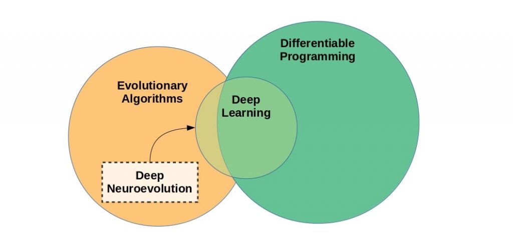
Deep learning can be categorized as a subspace of the more general differentiable programming. Deep neuroevolution refers to the optimization of neural networks by selection, without explicit differentiation or gradient descent.
Differentiable programming is a broader programming paradigm that encompasses most of deep learning, excepting gradient-free optimization methods such as neuroevolution/evolutionary algorithms. Yann LeCun, Chief AI Scientist at Facebook, touted the possibilities of differentiable programming in a Facebook post (content mirrored in a Github gist). To hear LeCun tell it, differentiable programming is little more than a rebranding of modern deep learning, incorporating dynamic definitions of neural networks with loops and conditionals.
I would argue that the consequences of widespread adoption of differentiable programming are closer to what Andrej Karpathy describes as “Software 2.0”, although he also limits his discussion largely to neural networks. It’s reasonable to argue that software 2.0/differentiable programming is a broader paradigm in its entirety than either LeCun or Karpathy described. Differentiable programming represents a generalization beyond the constraint of neural networks as function approximators to facilitate gradient-based optimization algorithms for a wide range of systems. If there is a Python library that is emblematic of the simplicity, flexibility, and utility of differentiable programming it has to be Autograd.
Combining Deep Learning with Differentiable Programming
Differentiating with respect to arbitrary physical simulations and mathematical primitives presents opportunities for solutions where deep neural networks are inefficient or ineffective. That’s not to say you should throw away all your deep learning intuition and experience. Rather, the most impressive solutions will combine elements of deep learning with the broader capabilities of differentiable programming, such as the work of Degrave et al. 2018, whose authors combined a differentiable physics engine with a neural network controller to solve robotic control tasks.
Essentially they extended the differentiable parts of the environment beyond the neural network to include simulated robot kinematics. They could then backpropagate through the parameters of the robot environment into the neural network policy, speeding up the optimization process by about 6x to 8x in terms of sample efficiency. They chose to use Theano as their automatic differentiation library, which prevented them from differentiating through conditional statements, limiting the types of contact constraints they could implement. A differentiable physics simulator built with Autograd or even recent versions of PyTorch or Tensorflow 2.0, which support differentiating through dynamic branching, would have even more possibilities for optimizing a neural network robot controller, e.g. offering more realistic collision detection.
The universal approximation power of deep neural networks makes them an incredible tool for problems in science, control, and data science, but sometimes this flexibility is more liability than utility, as anyone who has ever struggled with over-fitting can attest. As a famous quote from John von Neumann puts it: “With four parameters I can fit an elephant, and with five I can make him wiggle his trunk.” (an actual demonstration of this concept can be found in “Drawing an elephant with 4 complex parameters” by Mayer et al. [pdf]).
In modern machine learning practice, that means being careful not to mismatch your model to your dataset, a feat that for small datasets is all too easy to stumble into. In other words a big conv-net is likely to be overkill for many bespoke datasets with only a few hundred to a few thousand samples. In many physics problems, for example, it will be better to describe your problem mathematically and run gradient descent over the free parameters. Autograd is a Python package well suited to this approach, especially for Pythonicly-inclined mathematicians, physicists, and others who are well-practiced at describing problems at a low level with Python matrix and array computational package NumPy.
Autograd: Anything you can NumPy, you can differentiate
Here’s a simple example of what Autograd can do:
| import autograd.numpy as np from autograd import elementwise_grad as egrad import matplotlib.pyplot as plt x = np.linspace(-31.4,31.4, 256) sinc = lambda x: np.sin(x) / x plt.figure(figsize=(12,7)) plt.title(“sinc function and derivatives”, fontsize=24) my_fn = sinc for ii in range(9): plt.plot(x, my_fn(x), lw=3, label=”d{} sinc(x)/dx{}”.format(ii,ii)) plt.legend(fontsize=18) plt.axis([-32, 32, -0.50, 1.2]) plt.savefig(“./sinc_grad{}.png”.format(ii)) my_fn = egrad(my_fn) |
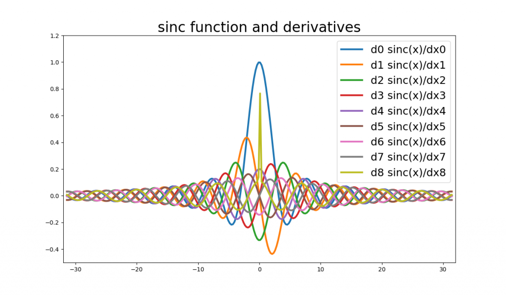
Differentiation with Autograd. In this case Autograd was able to differentiate up to the 7th derivative before running into some numerical stability problems around x=0 (note the sharp olive green spike in the center of the figure).
Autograd is a powerful automatic differentiation library that makes it possible to differentiate native Python and NumPy code. Derivatives can be computed to an arbitrary order (you can take derivatives of derivatives of derivatives, and so on), and assigned to multiple arrays of parameters so long as the final output is a scalar (e.g. a loss function). The resulting code is Pythonic, a.k.a. it is readable and maintainable, and it doesn’t require learning new syntax or style. That means we don’t have to worry about memorizing complex APIs like the contents of torch.nn or tf.keras.layers, and we can concentrate on the details of our problem, e.g. translating mathematics into code. Autograd+NumPy is a mature library that is maintained but no longer developed, so there’s no real danger of future updates breaking your project.
You can implement a neural network easily with Autograd, as the mathematical primitives of dense neural layers (matrix multiplication) and convolution (you can easily use Fourier transforms for this, or use convolve2d from scipy) have relatively fast implementations in NumPy. To try out a simple MLP demonstration on scikit-learn’s diminutive digits dataset, download this Github gist, (you may also be interested in studying the official example in the autograd repository).
If you copy the gist and run it in a local virtual environment you’ll need to pip install both autograd, and scikit-learn, the latter for its digits dataset. Once all set up, running the code should yield progress reports like the following:
| epoch 10, training loss 2.89e+02, train acc: 5.64e-01, val loss 3.94e+02, val accuracy 4.75e-01 total time: 4.26, epoch time 0.38 epoch 20, training loss 8.79e+01, train acc: 8.09e-01, val loss 9.96e+01, val accuracy 7.99e-01 total time: 7.73, epoch time 0.33 epoch 30, training loss 4.54e+01, train acc: 9.20e-01, val loss 4.55e+01, val accuracy 9.39e-01 total time: 11.49, epoch time 0.35 … epoch 280, training loss 1.77e+01, train acc: 9.99e-01, val loss 1.39e+01, val accuracy 9.83e-01 total time: 110.70, epoch time 0.49 epoch 290, training loss 1.76e+01, train acc: 9.99e-01, val loss 1.39e+01, val accuracy 9.83e-01 total time: 115.41, epoch time 0.43 |
That’s a reasonably good result of 98.3% validation accuracy after just under two minutes of training. With a little tweaking of hyperparameters, you could probably push that performance to 100% accuracy or very near. Autograd handles this small dataset easily and efficiently (while Autograd and NumPy operations don’t run on the GPU, primitives like matrix multiply do take advantage of multiple cores). But if all you wanted to do was build a shallow MLP you could do so more quickly in terms of both development and computational time with a more mainstream and modern machine learning library.
There is some utility in building simple models at a low-level like this where control is prioritized or as a learning exercise, of course, but if a small dense neural network was the final goal we’d recommend you stick to PyTorch or TensorFlow for brevity and compatibility with hardware accelerators like GPUs. Instead let’s dive into something a bit more interesting: simulating an optical neural network. The following tutorial does involve a bit of physics and a fair bit of code: if that’s not your thing feel free to skip ahead to the next section where we’ll touch on some of Autograd’s limitations.
Simulating an Optical Neural Network with Autograd
Optical neural networks (ONNs) are an old idea, with the scientific journal Applied Optics running special issues on the topic in 1987 and again in 1993. The concept has recently been revisited by academics (e.g. Zuo et al. 2019) and by startups such as Optalysys, Fathom Computing, and Lightmatter and Lightelligence, the last two of which were spun out of the same lab at MIT by co-authors on a high-profile paper published in Nature.
Light is an attractive physical phenomenon for implementing neural networks due to the similarity in the mathematics used to describe both neural networks and optical propagation. Thanks to the Fourier Transform property of lenses and the convolution property of the Fourier transform, convolutional layers can be implemented with a perturbative element placed after 2 focal lengths and one lens away from an input plane (this is known as a 4f correlator) while a matrix multiply can be implemented by placing the element 2 focal lengths and 1 lens from that. But this isn’t an optics lecture, it’s a coding tutorial, so let’s see some code!
To install the necessary dependencies, activate your desired virtual environment with your environment manager of choice and use pip to install Autograd and scikit-image if you haven’t already.
| pip install autograd pip install scikit-image |
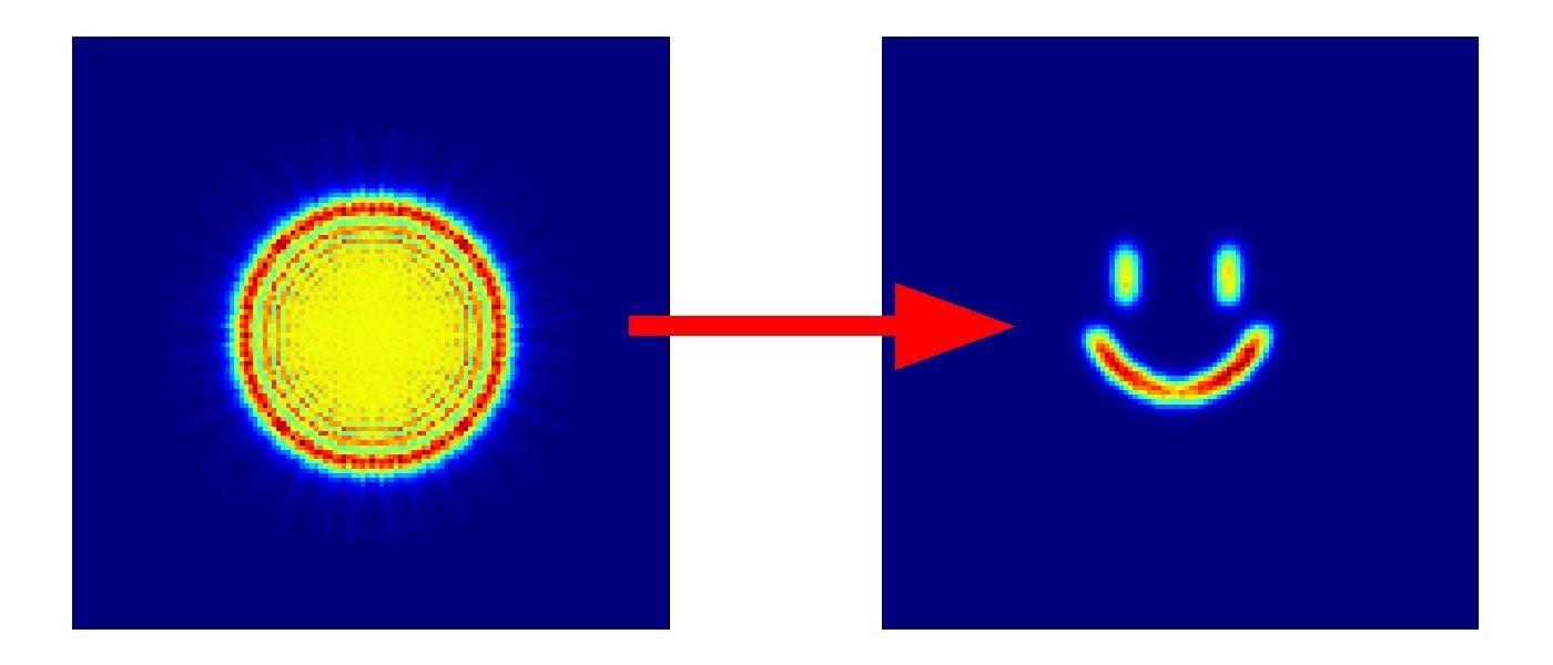
We’ll be simulating an optical system that essentially operates as a single-output generator, processing a flat input wavefront by passing it through a series of evenly-spaced phase images. To keep the tutorial relatively simple and the line count down, we will attempt to match only a single target image, shown below (you can download the image to your working directory if you want to follow along). After completing this simple tutorial, you may be inclined to experiment with building an optical classifier, autoencoder, or some other image transformation.

Now for some Python, starting with importing the packages we’ll need.
| import autograd.numpy as np from autograd import grad import matplotlib.pyplot as plt import time import skimage import skimage.io as sio |
We’ll use the angular spectrum method to simulate optical propagation. This is a good method for near-field conditions where the aperture size of your lens or beam is similar to the propagation distance. The following function executes angular spectrum method propagation given a starting wavefront and its dimensions, wavelength of light, and propagation distance.
| def asm_prop(wavefront, length=32.e-3, \ wavelength=550.e-9, distance=10.e-3): if len(wavefront.shape) == 2: dim_x, dim_y = wavefront.shape elif len(wavefront.shape) == 3: number_samples, dim_x, dim_y = wavefront.shape else: print(“only 2D wavefronts or array of 2D wavefronts supported”) assert dim_x == dim_y, “wavefront should be square” px = length / dim_x l2 = (1/wavelength)**2 fx = np.linspace(-1/(2*px), 1/(2*px) – 1/(dim_x*px), dim_x) fxx, fyy = np.meshgrid(fx,fx) q = l2 – fxx**2 – fyy**2 q[q<0] = 0.0 h = np.fft.fftshift(np.exp(1.j * 2 * np.pi * distance * np.sqrt(q))) fd_wavefront = np.fft.fft2(np.fft.fftshift(wavefront)) if len(wavefront.shape) == 3: fd_new_wavefront = h[np.newaxis,:,:] * fd_wavefront New_wavefront = np.fft.ifftshift(np.fft.ifft2(\ fd_new_wavefront))[:,:dim_x,:dim_x] else: fd_new_wavefront = h * fd_wavefront new_wavefront = np.fft.ifftshift(np.fft.ifft2(\ fd_new_wavefront))[:dim_x,:dim_x] return new_wavefront |
Instead of restricting our ONN to either convolution or matrix multiplication operations, we’ll propagate our beam through a series of evenly spaced phase object images. Physically, this is similar to shining a coherent beam of light through a series of thin, wavy glass plates, only in this case we’ll use Autograd to backpropagate through the system to design them so that they direct light from the input wavefront to match a given target pattern at the end. After passing through the phase elements, we’ll collect the light on the equivalent of an image sensor. This gives us a nice nonlinearity in the conversion from a complex field to real-valued intensity that we could use to build a more complex optical neural network by stacking several of these together.
Each layer is defined by passing through a series of phase images separated by short distances. This is described computationally as propagation over a short distance, followed by a thin phase plate (implemented as multiplication):
| def onn_layer(wavefront, phase_objects, d=100.e-3): for ii in range(len(phase_objects)): wavefront = asm_prop(wavefront * phase_objects[ii], distance=d) return wavefront |
The key to training a model in Autograd is in defining a function that returns a scalar loss. This loss function can then be wrapped in Autograd’s grad function to compute gradients. You can specify which argument contains the parameters to compute gradients for the argnum argument to grad, and remember that the loss function must return a single scalar value, not an array.
| def get_loss(wavefront, y_tgt, phase_objects, d=100.e-3): img = np.abs(onn_layer(wavefront, phase_objects, d=d))**2 mse_loss = np.mean( (img – y_tgt)**2 + np.abs(img-y_tgt) ) return mse_loss get_grad = grad(get_loss, argnum=2) |
First, let’s read in the target image and set up the input wavefront. Feel free to use a 64 by 64 image of your choosing, or download the grayscale smiley image from earlier in the article.
| # target image tgt_img = sio.imread(“./smiley.png”)[:, :, 0] y_tgt = 1.0 * tgt_img / np.max(tgt_img) # set up input wavefront (a flat plane wave with an 16mm aperture) dim = 128 side_length = 32.e-3 aperture = 8.e-3 wavelength = 550.e-9 k0 = 2*np.pi / wavelength px = side_length / dim x = np.linspace(-side_length/2, side_length/2-px, dim) xx, yy = np.meshgrid(x,x) rr = np.sqrt(xx**2 + yy**2) wavefront = np.zeros((dim,dim)) * np.exp(1.j*k0*0.0) wavefront[rr <= aperture] = 1.0 |
Next, define the learning rate, propagation distance, and the model parameters.
| lr = 1e-3 dist = 50.e-3 phase_objects = [np.exp(1.j * np.zeros((128,128))) \ for aa in range(32)] losses = [] |
If you’re familiar with training neural networks with PyTorch or similar librarie
| for step in range(128): my_grad = get_grad(wavefront, y_tgt, phase_objects, d=dist) for params, grads in zip(phase_objects, my_grad): params -= lr * np.exp( -1.j * np.angle(grads)) loss = get_loss(wavefront, y_tgt, phase_objects,d=dist) losses.append(loss) img = np.abs(onn_layer(wavefront, phase_objects))**2 print(“loss at step {} = {:.2e}, lr={:.3e}”.format(step, loss, lr)) fig = plt.figure(figsize=(12,7)) plt.imshow(img / 2.0, cmap=”jet”) plt.savefig(“./smiley_img{}.png”.format(step)) plt.close(fig) fig = plt.figure(figsize=(7,4)) plt.plot(losses, lw=3) plt.savefig(“./smiley_losses.png”) |
If everything worked out you should see monotonically decreasing mean squared error loss and the code will save a series of figures depicting optical network’s output as it gets closer and closer to matching the target image.
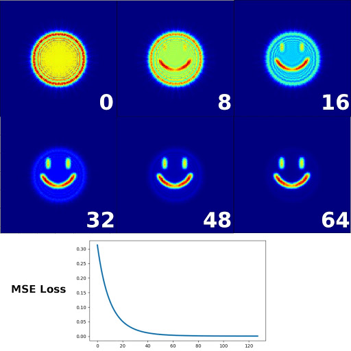
Optimization of the optical system attempting to match the target image. Each of the numbered images with a blue background is the model output at different training steps. Unsurprisingly for training with a single sample, the loss decreases smoothly over the course of training.
That’s it! We’ve simulated an optical system acting as a single-output generator. If you have any trouble getting the code to run, try copying the code from this Github gist all in one go to prevent introducing typos.
Autograd Uses and Limitations
Autograd is a flexible automatic differentiation package that has influenced mainstream machine learning libraries in many ways. It’s not always easy to determine the ancestry of how different ideas influence one another in a rapidly developing space like machine learning. However, the imperative, define-by-run approach features prominently in Chainer, PyTorch, and to some extent TensorFlow versions after 2.0 that feature eager execution. According to libraries.io ten other Python packages depend on Autograd, including packages for solving inverse kinematics, sensitivity analysis, and Gaussian processes. My personal favorite is the quantum machine learning package PennyLane.
Autograd may not be as powerful as PyTorch or TensorFlow, and it doesn’t have implementations of all the latest deep learning tricks, but in some ways this can be an advantage during certain stages of development. There aren’t a lot of specialized APIs to memorize and the learning curve is particularly gentle for anyone who is familiar with Python and/or NumPy. It doesn’t have any of the bells and whistles for deployment or scaling, but it is simple and efficient to use for projects where control and customization is important. It’s particularly well-suited to mathematicians and physicists who need to translate abstract ideas from math to code to build arbitrary machine learning or optimization solutions at a low-level of implementation.
The biggest con to using Autograd in our opinion is a lack of support for hardware acceleration. Perhaps there’s no better way to describe this drawback than the 4-year-long discussion on this Github issue, which discusses various ways of introducing GPU support. If you worked your way through the optical neural network tutorial in this post you’ll have already noticed that running an experiment with even a modestly sized model could require a prohibitively high amount of computational time. Computation speed with Autograd is enough of a drawback that we don’t actually recommend using it for projects much larger than the MLP or ONN generator demonstrations described above.
Instead, consider JAX, an Apache 2.0 licensed library developed by Google Brain researchers, including the Autograd developers. JAX combines hardware acceleration and just-in-time compilation for substantial speedups over native NumPy code, and in addition, JAX offers a set of function transformations for automatically parallelizing code. JAX can be slightly more complicated than a direct NumPy replacement with Autograd, but its powerful features can more than make up for that. We’ll compare JAX to Autograd as well as the popular PyTorch and TensorFlow in a future article.
Have any questions about Autograd, other machine learning libraries, or systems that can support them?
Contact Exxact Today

Autograd: The Best Machine Learning Library You’re Not Using?
Autograd: The Missing Machine Learning Library
Wait, people use libraries other than TensorFlow and PyTorch?
Ask a group of deep learning practitioners for their programming language of choice and you’ll undoubtedly hear a lot about Python. Ask about their go-to machine learning library, on the other hand, and you’re likely to get a picture of a two library system with a mix of TensorFlow and PyTorch. While there are plenty of people that may be familiar with both, in general commercial applications in machine learning (ML) tend to be dominated by the use of TensorFlow, while research projects in artificial intelligence/ML mostly use PyTorch. Although there’s significant convergence between the two libraries with the introduction of eager execution by default in TensorFlow 2.0 released last year, and the availability of building static executable models using Torchscript, most seem to stick to one or the other for the most part.
While the general consensus seems to be that you should pick TensorFlow for its better deployment and edge support if you want to join a company, and PyTorch for flexibility and readability if you want to work in academic research, there’s more to the world of AI/ML libraries than just PyTorch and TensorFlow. Just like there’s more to AI/ML than just deep learning. In fact, the gradients and tensor computations powering deep learning promise to have a wide-ranging impact in fields ranging from physics to biology. While we would bet that the so-called shortage of ML/AI researchers is exaggerated (and who wants to dedicate their most creative years to maximizing ad engagement and recommending more addictive newsfeeds?), we expect that the tools of differentiable programming will be increasingly valuable to a wide variety of professionals for the foreseeable future.
Differentiable Computing is Bigger than Deep Learning
Deep learning, the use of many-layered artificial neural networks very loosely based on ideas about computation in mammalian brains, is well known for its impacts on fields like computer vision and natural language processing. We’ve also seen that many of the lessons in hardware and software developed alongside deep learning in the past decade (gradient descent, function approximation, and accelerated tensor computations) have found interesting applications in the absence of neural networks.
Interested in getting faster results?
Learn more about Exxact Deep Learning Solutions
Automatic differentiation and gradient descent over the parameters of quantum circuits offers meaningful utility for quantum computing in the era of Noisy Intermediate-Scale Quantum (NISQ) computing devices (i.e. quantum computing devices that are available now). The penultimate step in DeepMind’s impressive upset at the CASP13 protein folding prediction conference and competition used gradient descent applied directly over predicted amino acid positions, rather than a deep neural network as the Google Alphabet subsidiary is well known for. These are just a few examples of the power of differentiable programming unbound by the paradigm of artificial neurons.

Deep learning can be categorized as a subspace of the more general differentiable programming. Deep neuroevolution refers to the optimization of neural networks by selection, without explicit differentiation or gradient descent.
Differentiable programming is a broader programming paradigm that encompasses most of deep learning, excepting gradient-free optimization methods such as neuroevolution/evolutionary algorithms. Yann LeCun, Chief AI Scientist at Facebook, touted the possibilities of differentiable programming in a Facebook post (content mirrored in a Github gist). To hear LeCun tell it, differentiable programming is little more than a rebranding of modern deep learning, incorporating dynamic definitions of neural networks with loops and conditionals.
I would argue that the consequences of widespread adoption of differentiable programming are closer to what Andrej Karpathy describes as “Software 2.0”, although he also limits his discussion largely to neural networks. It’s reasonable to argue that software 2.0/differentiable programming is a broader paradigm in its entirety than either LeCun or Karpathy described. Differentiable programming represents a generalization beyond the constraint of neural networks as function approximators to facilitate gradient-based optimization algorithms for a wide range of systems. If there is a Python library that is emblematic of the simplicity, flexibility, and utility of differentiable programming it has to be Autograd.
Combining Deep Learning with Differentiable Programming
Differentiating with respect to arbitrary physical simulations and mathematical primitives presents opportunities for solutions where deep neural networks are inefficient or ineffective. That’s not to say you should throw away all your deep learning intuition and experience. Rather, the most impressive solutions will combine elements of deep learning with the broader capabilities of differentiable programming, such as the work of Degrave et al. 2018, whose authors combined a differentiable physics engine with a neural network controller to solve robotic control tasks.
Essentially they extended the differentiable parts of the environment beyond the neural network to include simulated robot kinematics. They could then backpropagate through the parameters of the robot environment into the neural network policy, speeding up the optimization process by about 6x to 8x in terms of sample efficiency. They chose to use Theano as their automatic differentiation library, which prevented them from differentiating through conditional statements, limiting the types of contact constraints they could implement. A differentiable physics simulator built with Autograd or even recent versions of PyTorch or Tensorflow 2.0, which support differentiating through dynamic branching, would have even more possibilities for optimizing a neural network robot controller, e.g. offering more realistic collision detection.
The universal approximation power of deep neural networks makes them an incredible tool for problems in science, control, and data science, but sometimes this flexibility is more liability than utility, as anyone who has ever struggled with over-fitting can attest. As a famous quote from John von Neumann puts it: “With four parameters I can fit an elephant, and with five I can make him wiggle his trunk.” (an actual demonstration of this concept can be found in “Drawing an elephant with 4 complex parameters” by Mayer et al. [pdf]).
In modern machine learning practice, that means being careful not to mismatch your model to your dataset, a feat that for small datasets is all too easy to stumble into. In other words a big conv-net is likely to be overkill for many bespoke datasets with only a few hundred to a few thousand samples. In many physics problems, for example, it will be better to describe your problem mathematically and run gradient descent over the free parameters. Autograd is a Python package well suited to this approach, especially for Pythonicly-inclined mathematicians, physicists, and others who are well-practiced at describing problems at a low level with Python matrix and array computational package NumPy.
Autograd: Anything you can NumPy, you can differentiate
Here’s a simple example of what Autograd can do:
| import autograd.numpy as np from autograd import elementwise_grad as egrad import matplotlib.pyplot as plt x = np.linspace(-31.4,31.4, 256) sinc = lambda x: np.sin(x) / x plt.figure(figsize=(12,7)) plt.title(“sinc function and derivatives”, fontsize=24) my_fn = sinc for ii in range(9): plt.plot(x, my_fn(x), lw=3, label=”d{} sinc(x)/dx{}”.format(ii,ii)) plt.legend(fontsize=18) plt.axis([-32, 32, -0.50, 1.2]) plt.savefig(“./sinc_grad{}.png”.format(ii)) my_fn = egrad(my_fn) |

Differentiation with Autograd. In this case Autograd was able to differentiate up to the 7th derivative before running into some numerical stability problems around x=0 (note the sharp olive green spike in the center of the figure).
Autograd is a powerful automatic differentiation library that makes it possible to differentiate native Python and NumPy code. Derivatives can be computed to an arbitrary order (you can take derivatives of derivatives of derivatives, and so on), and assigned to multiple arrays of parameters so long as the final output is a scalar (e.g. a loss function). The resulting code is Pythonic, a.k.a. it is readable and maintainable, and it doesn’t require learning new syntax or style. That means we don’t have to worry about memorizing complex APIs like the contents of torch.nn or tf.keras.layers, and we can concentrate on the details of our problem, e.g. translating mathematics into code. Autograd+NumPy is a mature library that is maintained but no longer developed, so there’s no real danger of future updates breaking your project.
You can implement a neural network easily with Autograd, as the mathematical primitives of dense neural layers (matrix multiplication) and convolution (you can easily use Fourier transforms for this, or use convolve2d from scipy) have relatively fast implementations in NumPy. To try out a simple MLP demonstration on scikit-learn’s diminutive digits dataset, download this Github gist, (you may also be interested in studying the official example in the autograd repository).
If you copy the gist and run it in a local virtual environment you’ll need to pip install both autograd, and scikit-learn, the latter for its digits dataset. Once all set up, running the code should yield progress reports like the following:
| epoch 10, training loss 2.89e+02, train acc: 5.64e-01, val loss 3.94e+02, val accuracy 4.75e-01 total time: 4.26, epoch time 0.38 epoch 20, training loss 8.79e+01, train acc: 8.09e-01, val loss 9.96e+01, val accuracy 7.99e-01 total time: 7.73, epoch time 0.33 epoch 30, training loss 4.54e+01, train acc: 9.20e-01, val loss 4.55e+01, val accuracy 9.39e-01 total time: 11.49, epoch time 0.35 … epoch 280, training loss 1.77e+01, train acc: 9.99e-01, val loss 1.39e+01, val accuracy 9.83e-01 total time: 110.70, epoch time 0.49 epoch 290, training loss 1.76e+01, train acc: 9.99e-01, val loss 1.39e+01, val accuracy 9.83e-01 total time: 115.41, epoch time 0.43 |
That’s a reasonably good result of 98.3% validation accuracy after just under two minutes of training. With a little tweaking of hyperparameters, you could probably push that performance to 100% accuracy or very near. Autograd handles this small dataset easily and efficiently (while Autograd and NumPy operations don’t run on the GPU, primitives like matrix multiply do take advantage of multiple cores). But if all you wanted to do was build a shallow MLP you could do so more quickly in terms of both development and computational time with a more mainstream and modern machine learning library.
There is some utility in building simple models at a low-level like this where control is prioritized or as a learning exercise, of course, but if a small dense neural network was the final goal we’d recommend you stick to PyTorch or TensorFlow for brevity and compatibility with hardware accelerators like GPUs. Instead let’s dive into something a bit more interesting: simulating an optical neural network. The following tutorial does involve a bit of physics and a fair bit of code: if that’s not your thing feel free to skip ahead to the next section where we’ll touch on some of Autograd’s limitations.
Simulating an Optical Neural Network with Autograd
Optical neural networks (ONNs) are an old idea, with the scientific journal Applied Optics running special issues on the topic in 1987 and again in 1993. The concept has recently been revisited by academics (e.g. Zuo et al. 2019) and by startups such as Optalysys, Fathom Computing, and Lightmatter and Lightelligence, the last two of which were spun out of the same lab at MIT by co-authors on a high-profile paper published in Nature.
Light is an attractive physical phenomenon for implementing neural networks due to the similarity in the mathematics used to describe both neural networks and optical propagation. Thanks to the Fourier Transform property of lenses and the convolution property of the Fourier transform, convolutional layers can be implemented with a perturbative element placed after 2 focal lengths and one lens away from an input plane (this is known as a 4f correlator) while a matrix multiply can be implemented by placing the element 2 focal lengths and 1 lens from that. But this isn’t an optics lecture, it’s a coding tutorial, so let’s see some code!
To install the necessary dependencies, activate your desired virtual environment with your environment manager of choice and use pip to install Autograd and scikit-image if you haven’t already.
| pip install autograd pip install scikit-image |
We’ll be simulating an optical system that essentially operates as a single-output generator, processing a flat input wavefront by passing it through a series of evenly-spaced phase images. To keep the tutorial relatively simple and the line count down, we will attempt to match only a single target image, shown below (you can download the image to your working directory if you want to follow along). After completing this simple tutorial, you may be inclined to experiment with building an optical classifier, autoencoder, or some other image transformation.

Now for some Python, starting with importing the packages we’ll need.
| import autograd.numpy as np from autograd import grad import matplotlib.pyplot as plt import time import skimage import skimage.io as sio |
We’ll use the angular spectrum method to simulate optical propagation. This is a good method for near-field conditions where the aperture size of your lens or beam is similar to the propagation distance. The following function executes angular spectrum method propagation given a starting wavefront and its dimensions, wavelength of light, and propagation distance.
| def asm_prop(wavefront, length=32.e-3, \ wavelength=550.e-9, distance=10.e-3): if len(wavefront.shape) == 2: dim_x, dim_y = wavefront.shape elif len(wavefront.shape) == 3: number_samples, dim_x, dim_y = wavefront.shape else: print(“only 2D wavefronts or array of 2D wavefronts supported”) assert dim_x == dim_y, “wavefront should be square” px = length / dim_x l2 = (1/wavelength)**2 fx = np.linspace(-1/(2*px), 1/(2*px) – 1/(dim_x*px), dim_x) fxx, fyy = np.meshgrid(fx,fx) q = l2 – fxx**2 – fyy**2 q[q<0] = 0.0 h = np.fft.fftshift(np.exp(1.j * 2 * np.pi * distance * np.sqrt(q))) fd_wavefront = np.fft.fft2(np.fft.fftshift(wavefront)) if len(wavefront.shape) == 3: fd_new_wavefront = h[np.newaxis,:,:] * fd_wavefront New_wavefront = np.fft.ifftshift(np.fft.ifft2(\ fd_new_wavefront))[:,:dim_x,:dim_x] else: fd_new_wavefront = h * fd_wavefront new_wavefront = np.fft.ifftshift(np.fft.ifft2(\ fd_new_wavefront))[:dim_x,:dim_x] return new_wavefront |
Instead of restricting our ONN to either convolution or matrix multiplication operations, we’ll propagate our beam through a series of evenly spaced phase object images. Physically, this is similar to shining a coherent beam of light through a series of thin, wavy glass plates, only in this case we’ll use Autograd to backpropagate through the system to design them so that they direct light from the input wavefront to match a given target pattern at the end. After passing through the phase elements, we’ll collect the light on the equivalent of an image sensor. This gives us a nice nonlinearity in the conversion from a complex field to real-valued intensity that we could use to build a more complex optical neural network by stacking several of these together.
Each layer is defined by passing through a series of phase images separated by short distances. This is described computationally as propagation over a short distance, followed by a thin phase plate (implemented as multiplication):
| def onn_layer(wavefront, phase_objects, d=100.e-3): for ii in range(len(phase_objects)): wavefront = asm_prop(wavefront * phase_objects[ii], distance=d) return wavefront |
The key to training a model in Autograd is in defining a function that returns a scalar loss. This loss function can then be wrapped in Autograd’s grad function to compute gradients. You can specify which argument contains the parameters to compute gradients for the argnum argument to grad, and remember that the loss function must return a single scalar value, not an array.
| def get_loss(wavefront, y_tgt, phase_objects, d=100.e-3): img = np.abs(onn_layer(wavefront, phase_objects, d=d))**2 mse_loss = np.mean( (img – y_tgt)**2 + np.abs(img-y_tgt) ) return mse_loss get_grad = grad(get_loss, argnum=2) |
First, let’s read in the target image and set up the input wavefront. Feel free to use a 64 by 64 image of your choosing, or download the grayscale smiley image from earlier in the article.
| # target image tgt_img = sio.imread(“./smiley.png”)[:, :, 0] y_tgt = 1.0 * tgt_img / np.max(tgt_img) # set up input wavefront (a flat plane wave with an 16mm aperture) dim = 128 side_length = 32.e-3 aperture = 8.e-3 wavelength = 550.e-9 k0 = 2*np.pi / wavelength px = side_length / dim x = np.linspace(-side_length/2, side_length/2-px, dim) xx, yy = np.meshgrid(x,x) rr = np.sqrt(xx**2 + yy**2) wavefront = np.zeros((dim,dim)) * np.exp(1.j*k0*0.0) wavefront[rr <= aperture] = 1.0 |
Next, define the learning rate, propagation distance, and the model parameters.
| lr = 1e-3 dist = 50.e-3 phase_objects = [np.exp(1.j * np.zeros((128,128))) \ for aa in range(32)] losses = [] |
If you’re familiar with training neural networks with PyTorch or similar librarie
| for step in range(128): my_grad = get_grad(wavefront, y_tgt, phase_objects, d=dist) for params, grads in zip(phase_objects, my_grad): params -= lr * np.exp( -1.j * np.angle(grads)) loss = get_loss(wavefront, y_tgt, phase_objects,d=dist) losses.append(loss) img = np.abs(onn_layer(wavefront, phase_objects))**2 print(“loss at step {} = {:.2e}, lr={:.3e}”.format(step, loss, lr)) fig = plt.figure(figsize=(12,7)) plt.imshow(img / 2.0, cmap=”jet”) plt.savefig(“./smiley_img{}.png”.format(step)) plt.close(fig) fig = plt.figure(figsize=(7,4)) plt.plot(losses, lw=3) plt.savefig(“./smiley_losses.png”) |
If everything worked out you should see monotonically decreasing mean squared error loss and the code will save a series of figures depicting optical network’s output as it gets closer and closer to matching the target image.

Optimization of the optical system attempting to match the target image. Each of the numbered images with a blue background is the model output at different training steps. Unsurprisingly for training with a single sample, the loss decreases smoothly over the course of training.
That’s it! We’ve simulated an optical system acting as a single-output generator. If you have any trouble getting the code to run, try copying the code from this Github gist all in one go to prevent introducing typos.
Autograd Uses and Limitations
Autograd is a flexible automatic differentiation package that has influenced mainstream machine learning libraries in many ways. It’s not always easy to determine the ancestry of how different ideas influence one another in a rapidly developing space like machine learning. However, the imperative, define-by-run approach features prominently in Chainer, PyTorch, and to some extent TensorFlow versions after 2.0 that feature eager execution. According to libraries.io ten other Python packages depend on Autograd, including packages for solving inverse kinematics, sensitivity analysis, and Gaussian processes. My personal favorite is the quantum machine learning package PennyLane.
Autograd may not be as powerful as PyTorch or TensorFlow, and it doesn’t have implementations of all the latest deep learning tricks, but in some ways this can be an advantage during certain stages of development. There aren’t a lot of specialized APIs to memorize and the learning curve is particularly gentle for anyone who is familiar with Python and/or NumPy. It doesn’t have any of the bells and whistles for deployment or scaling, but it is simple and efficient to use for projects where control and customization is important. It’s particularly well-suited to mathematicians and physicists who need to translate abstract ideas from math to code to build arbitrary machine learning or optimization solutions at a low-level of implementation.
The biggest con to using Autograd in our opinion is a lack of support for hardware acceleration. Perhaps there’s no better way to describe this drawback than the 4-year-long discussion on this Github issue, which discusses various ways of introducing GPU support. If you worked your way through the optical neural network tutorial in this post you’ll have already noticed that running an experiment with even a modestly sized model could require a prohibitively high amount of computational time. Computation speed with Autograd is enough of a drawback that we don’t actually recommend using it for projects much larger than the MLP or ONN generator demonstrations described above.
Instead, consider JAX, an Apache 2.0 licensed library developed by Google Brain researchers, including the Autograd developers. JAX combines hardware acceleration and just-in-time compilation for substantial speedups over native NumPy code, and in addition, JAX offers a set of function transformations for automatically parallelizing code. JAX can be slightly more complicated than a direct NumPy replacement with Autograd, but its powerful features can more than make up for that. We’ll compare JAX to Autograd as well as the popular PyTorch and TensorFlow in a future article.
Have any questions about Autograd, other machine learning libraries, or systems that can support them?
Contact Exxact Today


