Artificial Intelligence
Save, Load, & Checkpoint Deep Learning Model in Keras
January 4, 2024
20 min read


Training a deep neural network can sometimes end as fast as it began. Or worse, the training run diverged! Here’s a familiar scenario: we start to get a robust learning curve with monotonically decreasing loss and little to no divergence in training and test set performance, make a few clever changes only to find the training collapses.
If we don’t have a checkpoint logged from when things were going swell, we’ll definitely wish we had. For this, we will need a strategy for logging checkpoints that fits your scenario. Keras, the high-level API for TensorFlow, makes keeping track of model versions easy with a built-in checkpoint callback. There are still trade-offs to logging too many checkpoints, however, and some scenarios where users will still want to use manual saves for their model.
In this article, we’ll discuss the three main ways to save and restore models when working with Keras, with examples and discussions on when and why to choose each one.
For this tutorial, we’ll use a simple image classification training run as a test bed for experimenting with different methods for saving, loading, and automatically logging checkpoints during training. To make a new virtual environment to work with (using virtualenv on Linux):
virtualenv tf_checkpoints –python=python3.8
source tf_checkpoints/bin/activate
Readers who already have a TensorFlow 2.xx virtual environment set up can simply activate that and get started right away. The only dependencies are as follows:
pip install tensorflow tensorflow_datasets matplotlib jupyter
# only needed to save the model in TensorFlow JS format
pip install tensorflowjs
Feel free to pull all the code we’ll go through in the examples from the repository on GitHub:
git clone git@github.com:riveSunder/tf_keras_checkpoints.git
It is also possible to run the code for this tutorial from start to finish as a Jupyter notebook hosted on Kaggle. This is a good option for readers who don’t have a local GPU available to train on but does require a Kaggle account. The datasets we are using are small enough to train on a laptop, albeit not as quickly as with a GPU available.
First, we’ll go through the common framework that we’ll use for training with all the different checkpoint methods we’ll go over later. First, imports:
import os
import numpy as np
import tensorflow as tf

from tensorflow.keras.models import Sequential
from tensorflow.keras.layers import Dense,\
  Dropout, \
  ELU, \
  Softmax, \
  Flatten
import tensorflow_datasets as tfds
import matplotlib.pyplot as plt
Next, we have a minimal number of hyperparameters that can be changed if needed. By default, we are using one of the simpler datasets provided in TensorFlow Datasets. These datasets can be trained quickly and easily, so we’ll be able to focus on the topic at hand: checkpoints.
model_iteration = 0
number_epochs = 32
batch_size = 2
my_lr = 3e-4
easy_mode = False

if easy_mode:
  dataset_name = "rock_paper_scissors"
else:
  dataset_name = "beans"

model_name = "mobilenet"
The “rock_paper_scissors” and “beans” datasets are small and simple enough for training a basic model to high accuracy in the high 0.90s with short training runs, perfect for our needs. We’ll use MobileNet, a particularly efficient model that has only a few million parameters, with pre-trained weights as our starting point.
The _PrefetchDataset object from tensorflow_datasets doesn’t slot directly into the fit method for Keras Models, so we’ll convert it to a form that does. The helper function tfds_to_numpy takes as input a _PrefetchDataset object and returns the input data and output labels as numpy arrays. Note that this shortcut is convenient for our tutorial, but it relies on the dataset being small enough to fit into memory.
def tfds_to_numpy(dataset):
  train_np_iterator = tfds.as_numpy(dataset)

  train_x = None
  train_y = None

  for elem in train_np_iterator:
  image = elem["image"].reshape(-1, *elem["image"].shape)
  label = elem["label"].reshape(1)
  if train_x is None:
    train_x = image
    train_y = label
  else:
    train_x = np.append(train_x, image, 0)
    train_y = np.append(train_y, label, 0)
  return train_x, train_y
We will also use a helper function for instantiating models with a MobileNet base for feature extraction. To the base model, the helper function adds a top of 3 dense layers with exponential linear units. Note that the function takes the number of neural nodes per hidden layer as an input, so we can try models with different dense layer sizes. By default, the MobileNet base parameters are not trained.
def initialize_model(number_classes, \
  input_shape, hidden_dims=64, \
  my_lr=my_lr, trainable_base=False):

  tf.random.set_seed(13)
  np.random.seed(13)
  extractor = tf.keras.applications.MobileNet(\
    input_shape=input_shape, include_top=False,\
    weights="imagenet")

    # Set to True to also train the feature extraction layers
    extractor.trainable = trainable_base

    model = Sequential([extractor, \
      Flatten(), \
      Dropout(0.25), \
      Dense(hidden_dims, \
        kernel_regularizer=l2(3e-4),\
        bias_regularizer=l2(1e-3)), \
      ELU(), \
      Dropout(0.25), \
      Dense(hidden_dims, \
        kernel_regularizer=l2(3e-4),\
        bias_regularizer=l2(1e-3)), \
      ELU(), \
      Dense(number_classes),
      Softmax()
      ])

example_output = model(np.random.rand(1,*input_shape))
my_loss = tf.keras.losses.SparseCategoricalCrossentropy()
model.compile(optimizer = "adam", \
  loss=my_loss, \
  metrics = ["accuracy"] \
  )

model.optimizer.lr = my_lr
return model
Another helper function provides a quick way to visualize training runs.
def visualize_history(history, save_figure=False):
  # Visualize Training
  my_cmap = plt.get_cmap("magma")
  loss_color = my_cmap(16)
  val_loss_color = my_cmap(64)

  my_cmap = plt.get_cmap("viridis")
  acc_color = my_cmap(128)
  val_acc_color = my_cmap(192)

  fig, ax = plt.subplots(1,1, figsize=(8,4))
  ax_twin = ax.twinx()

  ax.plot(history.history["loss"], \
    color=loss_color, label="training loss")
  ax.plot(history.history["val_loss"], \
    color=val_loss_color, label="validation loss")
  ax.set_ylabel("Loss")
  ax.set_yticks(np.arange(0,4.0,0.5))

  ax_twin.plot(history.history["accuracy"],\
    color=acc_color, label="training accuracy")
  ax_twin.plot(history.history["val_accuracy"], \
    color=val_acc_color, label="validation accuracy")
  ax_twin.set_ylabel("Accuracy")

  ax_twin.set_yticks(np.arange(0,1.0,0.1))
  ax.legend(loc=6)

  ax_twin.legend(loc=5)
  plt.show()
With our helper functions in place, we can now start setting up for training. We’ll use a few different directories to save models and model weights. If these don’t exist already, the following code will make them.
# Directory for saving model as SavedModel
saved_model_dir = os.path.join(\
  "..", "models",  f"{dataset_name}_{model_name}"\
    f"{model_iteration:03}")

if os.path.exists(saved_model_dir):
  while os.path.exists(saved_model_dir):
  model_iteration += 1
  saved_model_dir = os.path.join(\
    "..", "models",  f"{dataset_name}_{model_name}"\
    f"{model_iteration:03}")
else:
  os.system(f"mkdir {saved_model_dir} -p")

# Directory for saving model using BackupAndRestore
saved_backup_dir = os.path.join(\
  "..", "backups",  f"{dataset_name}_{model_name}\
    f"{model_iteration:03}")
if os.path.exists(saved_backup_dir):
  while os.path.exists(saved_backup_dir):
  model_iteration += 1
  saved_backup_dir = os.path.join(\
    "..", "backups",  f"{dataset_name}_{model_name}"\
    f"{model_iteration:03}")
else:
  os.system(f"mkdir {saved_backup_dir} -p")

saved_backup_path = os.path.join(saved_backup_dir,
"backup_{epoch:03d}_{val_loss:.2f}.ckpt")

# Directory for saving weights (only)
saved_weights_dir = os.path.join(\
  "..", "weights",  f"{dataset_name}_{model_name}"\
    f"{model_iteration:03}")

if os.path.exists(saved_weights_dir):
while os.path.exists(saved_weights_dir):
  model_iteration += 1
  saved_weights_dir = os.path.join(\
             "..", "weights",  f"{dataset_name}_{model_name}"\
f"{model_iteration:03}")

else:
  os.system(f"mkdir {saved_weights_dir} -p")
saved_weights_path = os.path.join(saved_weights_dir,
"checkpoint_{epoch:03d}_{val_loss:.2f}.hdf5")
Now we can start building callbacks to use with the fit method in Keras. In the first case, we won’t use any automatic checkpoint strategy, including only a learning rate scheduler and a tensorboard callback. This mimics the scenario where a deep learning practitioner may be in the early stages of building a model and training code and has skipped including checkpoint callbacks (relying on manually saving weights instead).
# Callbacks
# Defining a deliberately deleterious learning rate scheduler
def scheduler(epoch, lr, epochs=number_epochs):
  if epoch <= max([1, epochs - epochs // 4]):
  return lr * 0.9
  else:
  return lr * 20.

tensorboard_callback = tf.keras.callbacks.TensorBoard(\
  log_dir="logs", \
  write_graph=False, \
  update_freq='epoch', \
  )

lr_callback = tf.keras.callbacks.LearningRateScheduler(scheduler)
basic_callbacks = [tensorboard_callback, lr_callback]
Next, the dataset train and test splits are loaded from tensorflow_datasets. Then, we convert the _PrefetchDataset objects to numpy arrays.
train_dataset = tfds.load(dataset_name, split="train",
shuffle_files=True)
test_dataset = tfds.load(dataset_name, split="test",
shuffle_files=True)

test_x, test_y = tfds_to_numpy(test_dataset)
print(test_x.shape)
train_x, train_y = tfds_to_numpy(train_dataset)
print(train_x.shape)
Using a sample from the training dataset, we instantiate the model based on the input dimensions and number of labels in the training samples.
image = train_x[:1]
number_classes = np.max(train_y)+ 1
input_shape = image.shape[1:]

model = initialize_model(number_classes, input_shape)
model.summary()
The simplest strategy is to simply save model weights manually after training is complete. First, we initialize the model. The helper function we defined earlier returns a model that has already been compiled, so we can call the fit method right away. We’ll only train for 5 epochs for this first approach.
model = initialize_model(number_classes, input_shape)
history = model.fit(x=train_x, y=train_y, \
  validation_split=0.1, \
  batch_size=batch_size, epochs=5, \
  callbacks=basic_callbacks)
After the model trains to the last epoch, we can visualize training history for this run with our helper function:
visualize_history(history)
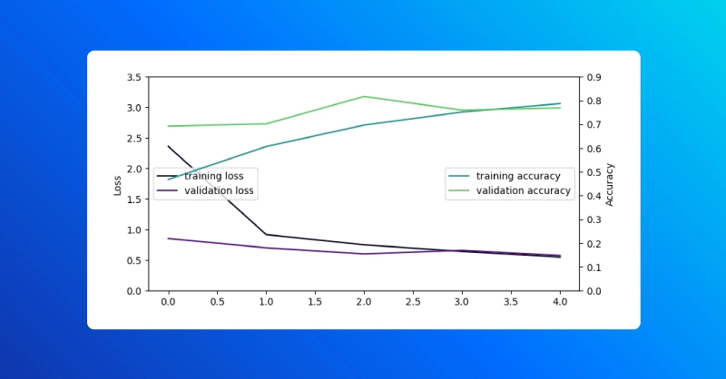
The save_weights and load_weights methods in the Keras Model class facilitate manually saving and loading model parameters. We then use the evaluate Model method to compare the model before and after loading the trained weights.
# Save model weights manually
weights_path = f"manual_weights{model_iteration:03}.ckpt"

model.save_weights(os.path.join(saved_weights_dir, weights_path))
loss, accuracy = model.evaluate(test_x, test_y, \
  batch_size=batch_size)

print(f"model loss: {loss:.3e},  accuracy: {accuracy:.3f}")
model = initialize_model(number_classes, input_shape)
loss, accuracy = model.evaluate(test_x, test_y, \
  batch_size=batch_size)
print(f"newly instantiated model loss: {loss:.3e},"\
  f"  accuracy: {accuracy:.3f}")
model.load_weights(os.path.join(saved_weights_dir, weights_path))
loss, accuracy = model.evaluate(test_x, test_y, \
  batch_size=batch_size)
print(f"model (weights loaded from disk) loss: {loss:.3e},"\
  f"  accuracy: {accuracy:.3f}")

"""
output:
64/64 [==============================] - 1s 11ms/step - loss: 0.4961 - accuracy: 0.8359
model loss: 4.961e-01,  accuracy: 0.836
64/64 [==============================] - 1s 10ms/step - loss: 1.8674 - accuracy: 0.2969
newly instantiated model loss: 1.867e+00,  accuracy: 0.297
64/64 [==============================] - 1s 10ms/step - loss: 0.4961 - accuracy: 0.8359
model (weights loaded from disk) loss: 4.961e-01,  accuracy: 0.836

"""
As you can see in the results returned from the evaluate method, they are the same after saving and loading parameters into a freshly instantiated model as they are for the original model immediately following training.
This manual method may be fine for the early stages of development, but as we’ll see in the next few sessions, there is a lot to be gained from using callbacks to automatically manage checkpoints.
One use case for logging checkpoints is recovering from an interrupted training session. This might be due to a keyboard interrupt (you forgot to add a crucial detail to the model before calling fit), power loss to your local workstation, a prematurely terminated spot instance in the cloud, or many other reasons.
The BackupAndRestore callback saves checkpoints (typically overwriting the old checkpoint each time) and allows your model to pick up where it left off.
# A callback to interrupt training,
# to demonstrate BackupAndRestore utility
class Interrupt(tf.keras.callbacks.Callback):
  def on_epoch_begin(self, epoch, logs=None):
    if epoch == 4:
      print("\n Interrupting callback")
      raise RuntimeError("Interrupting callback who?")

interrupt_callback = Interrupt()
callbacks_with_interrupt = basic_callbacks + [interrupt_callback]
model = initialize_model(number_classes, input_shape)

try:
  history = model.fit(x=train_x, y=train_y, \
  validation_split=0.1, \
  batch_size=batch_size, epochs=15, \
  callbacks=callbacks_with_interrupt)

except:
  pass
history = model.fit(x=train_x, y=train_y, \
  validation_split=0.1, \
  batch_size=batch_size, epochs=15, \
  callbacks=basic_callbacks)
"""
output:
…
Epoch 4/15
465/465 [==============================] - 6s 13ms/step - loss: 0.8091
- accuracy: 0.6828 - val_loss: 0.6051 - val_accuracy: 0.7500 - lr: 1.9683e-04
  Interrupting callback
Epoch 1/15
465/465 [==============================] - 6s 13ms/step - loss: 0.6791
- accuracy: 0.7624 - val_loss: 0.7334 - val_accuracy: 0.6923 - lr: 1.5943e-04
Epoch 2/15
465/465 [==============================] - 6s 13ms/step - loss: 0.5904
- accuracy: 0.7860 - val_loss: 0.7615 - val_accuracy: 0.7212 - lr: 1.4349e-04
Epoch 3/15
…
"""
We can see that after starting the fit method after the original fit call is interrupting by the callback, training starts over at epoch 1.
If we include the BackupAndRestore callback, training can pick up where it left off after being interrupted. The backup stored by this callback includes the optimizer state as well as storing the weights and remembering the epoch at which training left off.
number_batches = train_x.shape[0]
epoch_frequency = 3

# This is where we will define a BackupAndRestore callback
backup_callback = tf.keras.callbacks.BackupAndRestore( \
  saved_backup_dir, \
  save_freq = number_batches*epoch_frequency, \
  delete_checkpoint = True, \
  save_before_preemption = False
  )

callbacks_with_backup = callbacks_with_interrupt + [backup_callback]

model = initialize_model(number_labels, input_shape)

try:
  history = model.fit(x=train_x, y=train_y, \
  validation_split=0.1, \
  batch_size=batch_size, \
  epochs=5, \
  callbacks=callbacks_with_backup)

except:
  pass
history = model.fit(x=train_x, y=train_y, \
  validation_split=0.1, \
  batch_size=batch_size, \
  epochs=5, \
  callbacks=basic_callbacks)

"""
output:
…
Epoch 4/15
465/465 [==============================] - 6s 14ms/step - loss: 0.6736
- accuracy: 0.7022 - val_loss: 0.7657 - val_accuracy: 0.6538 - lr: 1.9683e-04
  Interrupting callback
Epoch 5/15
465/465 [==============================] - 6s 13ms/step - loss: 0.5869
- accuracy: 0.7656 - val_loss: 0.7563 - val_accuracy: 0.6154 - lr: 1.5943e-04
Epoch 6/15
465/465 [==============================] - 6s 13ms/step - loss: 0.4990
- accuracy: 0.7796 - val_loss: 0.9010 - val_accuracy: 0.6250 - lr: 1.4349e-04
Epoch 7/15
"""
Unlike the previous interrupted training run, the BackupAndRestore callback lets our model begin again from its last backup checkpoint.
The next method we’ll look at for saving and loading models is probably the most convenient, is mostly automatic, and will cover your needs for keeping track of model parameters during a large proportion of training scenarios.
This method relies on the ModelCheckpoint callback and works perfectly with the high-level fit API in Keras, with or without incorporating additional callbacks (such as the tensorboard callback for logging training info to a visual dashboard).
checkpoint_callback = tf.keras.callbacks.ModelCheckpoint(
saved_weights_path, \
save_freq = "epoch", \
monitor =  'val_accuracy', \
save_weights_only = True, \
verbose = 1)

callbacks_with_checkpoints = basic_callbacks + [checkpoint_callback]

model = initialize_model()

history = model.fit(x=train_x, y=train_y, \
     validation_split=0.1, \
     batch_size=batch_size, epochs=number_epochs, \
     callbacks=callbacks_with_checkpoints)

visualize_history(history)
The learning rate callback was intentionally sabotaged: after a certain number of epochs the learning rate grows instead of continuing to decay. As a result, loss explodes and the model becomes completely useless for its task.
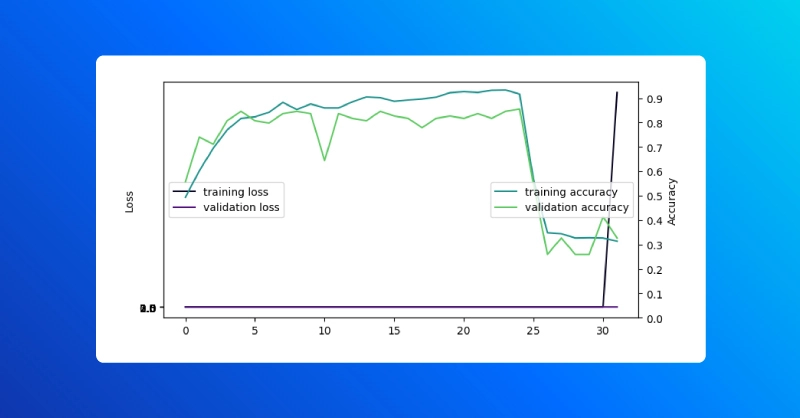
If we examine the training curve, we can pick out the last epoch with good performance, before the learning rate scheduler started increasing the learning rate. This kind of mistake could easily arise from a typo or other mistake (think multiplying by 20 Instead of dividing).
# Restore checkpoint with best performance

# add checkpoint with good performance
good_checkpoint = 24
chkpt_listdir = os.listdir(saved_weights_dir)

for elem in chkpt_listdir:
if f"checkpoint_{good_checkpoint:03}" in elem and "index" not in elem:
     print(elem)
     load_it = elem

loss, accuracy = model.evaluate(test_x, test_y, \
     batch_size=batch_size)

print(f"model (final training step) loss: {loss:.3e},  "\
f"accuracy: {accuracy:.3f}")

good_checkpoint_path = os.path.join(saved_weights_dir, load_it)
model.load_weights(good_checkpoint_path)

loss, accuracy = model.evaluate(test_x, test_y, \
     batch_size=batch_size)

print(f"model (loaded from last good checkpoint) loss: {loss:.3e}, "\
f"accuracy: {accuracy:.3f}")
"""
output:
checkpoint_024_0.94.hdf5
64/64 [==============================] - 1s 10ms/step - loss: 267607198400512.0000 - accuracy: 0.3359
model (final training step) loss: 2.676e+14,  accuracy: 0.336
64/64 [==============================] - 1s 10ms/step - loss: 0.6853 - accuracy: 0.8281
model (loaded from last good checkpoint) loss: 6.853e-01,  accuracy: 0.828
"""
When using the ModelCheckpoint callback to automatically log (weights only) checkpoints, you can easily restore a previously logged set of model parameters. That is, you can load the weights into a model that has the exact same architecture.
If, on the other hand, you have been experimenting with architectural hyperparameters and have a few different versions of your model saved to disk, some of these may not match up in the dimensions of each and every layer.
What happens if we try to load a previously logged checkpoint into a model that has almost, but not quite, the exact same architecture as before?
# Save model weights and architecture in SavedModel format
# If we change the model architecture
# but try to load the weights we saved before
wrong_model = initialize_model(number_classes, input_shape, hidden_dims=256)

print("Trying to load weights, into an architecture that does not match")
try:
wrong_model.load_weights(good_checkpoint_path)
except:
print(f"Model failed to load from {good_checkpoint_path}")
"""
output:
Trying to load weights, into an architecture that does not match
Model failed to load from ../weights/beans_mobilenet000/checkpoint_024_0.94.hdf5
"""
The model fails to load the weights we had saved previously. In this case, the number of nodes in each dense hidden layer did not match (256 versus 128), and the process throws an exception.
In situations like this, it can be useful to save the entire model in SavedModel format. When we save and load from the full model, we don’t run into problems instantiating the model with the wrong architecture for the parameters checkpoint.
model.save(saved_model_dir)
print("model saved")

loss, accuracy = model.evaluate(test_x, test_y, \
     batch_size=batch_size)

print(f"model that was saved to SavedModel directory, loss: "\
f"{loss:.3e},  accuracy: {accuracy:.3f}")

restored_model = tf.keras.models.load_model(saved_model_dir)
print("model restored")

loss, accuracy = restored_model.evaluate(test_x, test_y, \
     batch_size=batch_size)
print(f"restored from SavedModel directory, loss: {loss:.3e}, "\
f" accuracy: {accuracy:.3f}")

"""
output:
model saved
64/64 [==============================] - 1s 10ms/step - loss: 0.6853 - accuracy: 0.8281
model that was saved to SavedModel directory, loss: 6.853e-01,  accuracy: 0.828
model restored
64/64 [==============================] - 1s 10ms/step - loss: 0.6853 - accuracy: 0.8281
restored from SavedModel directory, loss: 6.853e-01,  accuracy: 0.828
"""
In addition to avoiding the problem with mis-specified architectures as demonstrated above, saving Keras models in SavedModel format enables a number of additional capabilities when moving models into production.
For example, we can convert a SavedModel to TensorFlow Lite format. TF Lite models take up less space on disk and utilize more efficient operators for inference, facilitating local execution on mobile phones and edge devices. An example of how to convert a Keras model from a SavedModel directory to make a TF Lite version is shown below.
We can then check to see if the model maintains its original performance using the evaluation loop below.
correct_lite = 0
total_samples = test_x.shape[0]

for my_index in range(test_x.shape[0]):

dtype = input_details[list(input_details.keys())[0]]["dtype"]
my_batch = np.array(test_x[my_index:my_index+1], dtype=dtype)

full_output_data = model(my_batch)
input_name = list(input_details.keys())[0]
output_name = list(output_details.keys())[0]

output_data = tf_lite_signature(**{input_name: my_batch})[output_name]

true_label = test_y[my_index]

correct_lite += 1.0 * (output_data.argmax() == true_label)

accuracy_lite = correct_lite / total_samples

print(f"TF Lite test accuracy: {accuracy_lite}")

"""
output:
TF Lite test accuracy: 0.828125
"""
For deploying small models to run in the browser, you may be interested in converting the Keras model into TensorFlow JavaScript format. This shards the model into smaller pieces and a format that can be used with JavaScript.
# to install tensorflowjs:
# ! pip install tensorflowjs
import tensorflowjs as tfjs

# convert from the keras model directly
tfjs.converters.save_keras_model(model, "tfjs_from_model")

# convert from the SavedModel directory
tfjs.converters.convert_tf_saved_model(saved_model_dir, "tfjs_from_saved_model")

# Check the contents of the tfjs directories
! ls tfjs_from_model
! ls tfjs_from_saved_model
Browser deployment with TensorFlow JS is beyond the scope of this tutorial, but for more information check out the official documentation.
In this article, we’ve explored several different approaches for saving training progress using manual saves and automatic checkpoint callbacks. Not only does an effective checkpoint strategy help to avoid the painful pitfalls of losing hard-earned training progress but saving models in the right format (such as SavedModel) can make iterative development and architecture exploration easier and can facilitate further refinement of models for deployment to edge devices or web browsers.
Training a deep learning model takes valuable time and losing progress can incur frustrating setbacks and longer time to completion. Exxact acknowledges the challenges and time it takes to develop and train these comprehensive models and offers a wide range of GPU accelerated workstations, servers, and full-scale solutions to help accelerate research. Contact us today for to learn more and get a formal quote on your next purpose-built customizable system.
Training a deep neural network can sometimes end as fast as it began. Or worse, the training run diverged! Here’s a familiar scenario: we start to get a robust learning curve with monotonically decreasing loss and little to no divergence in training and test set performance, make a few clever changes only to find the training collapses.
If we don’t have a checkpoint logged from when things were going swell, we’ll definitely wish we had. For this, we will need a strategy for logging checkpoints that fits your scenario. Keras, the high-level API for TensorFlow, makes keeping track of model versions easy with a built-in checkpoint callback. There are still trade-offs to logging too many checkpoints, however, and some scenarios where users will still want to use manual saves for their model.
In this article, we’ll discuss the three main ways to save and restore models when working with Keras, with examples and discussions on when and why to choose each one.
For this tutorial, we’ll use a simple image classification training run as a test bed for experimenting with different methods for saving, loading, and automatically logging checkpoints during training. To make a new virtual environment to work with (using virtualenv on Linux):
virtualenv tf_checkpoints –python=python3.8
source tf_checkpoints/bin/activate
Readers who already have a TensorFlow 2.xx virtual environment set up can simply activate that and get started right away. The only dependencies are as follows:
pip install tensorflow tensorflow_datasets matplotlib jupyter
# only needed to save the model in TensorFlow JS format
pip install tensorflowjs
Feel free to pull all the code we’ll go through in the examples from the repository on GitHub:
git clone git@github.com:riveSunder/tf_keras_checkpoints.git
It is also possible to run the code for this tutorial from start to finish as a Jupyter notebook hosted on Kaggle. This is a good option for readers who don’t have a local GPU available to train on but does require a Kaggle account. The datasets we are using are small enough to train on a laptop, albeit not as quickly as with a GPU available.
First, we’ll go through the common framework that we’ll use for training with all the different checkpoint methods we’ll go over later. First, imports:
import os
import numpy as np
import tensorflow as tf

from tensorflow.keras.models import Sequential
from tensorflow.keras.layers import Dense,\
  Dropout, \
  ELU, \
  Softmax, \
  Flatten
import tensorflow_datasets as tfds
import matplotlib.pyplot as plt
Next, we have a minimal number of hyperparameters that can be changed if needed. By default, we are using one of the simpler datasets provided in TensorFlow Datasets. These datasets can be trained quickly and easily, so we’ll be able to focus on the topic at hand: checkpoints.
model_iteration = 0
number_epochs = 32
batch_size = 2
my_lr = 3e-4
easy_mode = False

if easy_mode:
  dataset_name = "rock_paper_scissors"
else:
  dataset_name = "beans"

model_name = "mobilenet"
The “rock_paper_scissors” and “beans” datasets are small and simple enough for training a basic model to high accuracy in the high 0.90s with short training runs, perfect for our needs. We’ll use MobileNet, a particularly efficient model that has only a few million parameters, with pre-trained weights as our starting point.
The _PrefetchDataset object from tensorflow_datasets doesn’t slot directly into the fit method for Keras Models, so we’ll convert it to a form that does. The helper function tfds_to_numpy takes as input a _PrefetchDataset object and returns the input data and output labels as numpy arrays. Note that this shortcut is convenient for our tutorial, but it relies on the dataset being small enough to fit into memory.
def tfds_to_numpy(dataset):
  train_np_iterator = tfds.as_numpy(dataset)

  train_x = None
  train_y = None

  for elem in train_np_iterator:
  image = elem["image"].reshape(-1, *elem["image"].shape)
  label = elem["label"].reshape(1)
  if train_x is None:
    train_x = image
    train_y = label
  else:
    train_x = np.append(train_x, image, 0)
    train_y = np.append(train_y, label, 0)
  return train_x, train_y
We will also use a helper function for instantiating models with a MobileNet base for feature extraction. To the base model, the helper function adds a top of 3 dense layers with exponential linear units. Note that the function takes the number of neural nodes per hidden layer as an input, so we can try models with different dense layer sizes. By default, the MobileNet base parameters are not trained.
def initialize_model(number_classes, \
  input_shape, hidden_dims=64, \
  my_lr=my_lr, trainable_base=False):

  tf.random.set_seed(13)
  np.random.seed(13)
  extractor = tf.keras.applications.MobileNet(\
    input_shape=input_shape, include_top=False,\
    weights="imagenet")

    # Set to True to also train the feature extraction layers
    extractor.trainable = trainable_base

    model = Sequential([extractor, \
      Flatten(), \
      Dropout(0.25), \
      Dense(hidden_dims, \
        kernel_regularizer=l2(3e-4),\
        bias_regularizer=l2(1e-3)), \
      ELU(), \
      Dropout(0.25), \
      Dense(hidden_dims, \
        kernel_regularizer=l2(3e-4),\
        bias_regularizer=l2(1e-3)), \
      ELU(), \
      Dense(number_classes),
      Softmax()
      ])

example_output = model(np.random.rand(1,*input_shape))
my_loss = tf.keras.losses.SparseCategoricalCrossentropy()
model.compile(optimizer = "adam", \
  loss=my_loss, \
  metrics = ["accuracy"] \
  )

model.optimizer.lr = my_lr
return model
Another helper function provides a quick way to visualize training runs.
def visualize_history(history, save_figure=False):
  # Visualize Training
  my_cmap = plt.get_cmap("magma")
  loss_color = my_cmap(16)
  val_loss_color = my_cmap(64)

  my_cmap = plt.get_cmap("viridis")
  acc_color = my_cmap(128)
  val_acc_color = my_cmap(192)

  fig, ax = plt.subplots(1,1, figsize=(8,4))
  ax_twin = ax.twinx()

  ax.plot(history.history["loss"], \
    color=loss_color, label="training loss")
  ax.plot(history.history["val_loss"], \
    color=val_loss_color, label="validation loss")
  ax.set_ylabel("Loss")
  ax.set_yticks(np.arange(0,4.0,0.5))

  ax_twin.plot(history.history["accuracy"],\
    color=acc_color, label="training accuracy")
  ax_twin.plot(history.history["val_accuracy"], \
    color=val_acc_color, label="validation accuracy")
  ax_twin.set_ylabel("Accuracy")

  ax_twin.set_yticks(np.arange(0,1.0,0.1))
  ax.legend(loc=6)

  ax_twin.legend(loc=5)
  plt.show()
With our helper functions in place, we can now start setting up for training. We’ll use a few different directories to save models and model weights. If these don’t exist already, the following code will make them.
# Directory for saving model as SavedModel
saved_model_dir = os.path.join(\
  "..", "models",  f"{dataset_name}_{model_name}"\
    f"{model_iteration:03}")

if os.path.exists(saved_model_dir):
  while os.path.exists(saved_model_dir):
  model_iteration += 1
  saved_model_dir = os.path.join(\
    "..", "models",  f"{dataset_name}_{model_name}"\
    f"{model_iteration:03}")
else:
  os.system(f"mkdir {saved_model_dir} -p")

# Directory for saving model using BackupAndRestore
saved_backup_dir = os.path.join(\
  "..", "backups",  f"{dataset_name}_{model_name}\
    f"{model_iteration:03}")
if os.path.exists(saved_backup_dir):
  while os.path.exists(saved_backup_dir):
  model_iteration += 1
  saved_backup_dir = os.path.join(\
    "..", "backups",  f"{dataset_name}_{model_name}"\
    f"{model_iteration:03}")
else:
  os.system(f"mkdir {saved_backup_dir} -p")

saved_backup_path = os.path.join(saved_backup_dir,
"backup_{epoch:03d}_{val_loss:.2f}.ckpt")

# Directory for saving weights (only)
saved_weights_dir = os.path.join(\
  "..", "weights",  f"{dataset_name}_{model_name}"\
    f"{model_iteration:03}")

if os.path.exists(saved_weights_dir):
while os.path.exists(saved_weights_dir):
  model_iteration += 1
  saved_weights_dir = os.path.join(\
             "..", "weights",  f"{dataset_name}_{model_name}"\
f"{model_iteration:03}")

else:
  os.system(f"mkdir {saved_weights_dir} -p")
saved_weights_path = os.path.join(saved_weights_dir,
"checkpoint_{epoch:03d}_{val_loss:.2f}.hdf5")
Now we can start building callbacks to use with the fit method in Keras. In the first case, we won’t use any automatic checkpoint strategy, including only a learning rate scheduler and a tensorboard callback. This mimics the scenario where a deep learning practitioner may be in the early stages of building a model and training code and has skipped including checkpoint callbacks (relying on manually saving weights instead).
# Callbacks
# Defining a deliberately deleterious learning rate scheduler
def scheduler(epoch, lr, epochs=number_epochs):
  if epoch <= max([1, epochs - epochs // 4]):
  return lr * 0.9
  else:
  return lr * 20.

tensorboard_callback = tf.keras.callbacks.TensorBoard(\
  log_dir="logs", \
  write_graph=False, \
  update_freq='epoch', \
  )

lr_callback = tf.keras.callbacks.LearningRateScheduler(scheduler)
basic_callbacks = [tensorboard_callback, lr_callback]
Next, the dataset train and test splits are loaded from tensorflow_datasets. Then, we convert the _PrefetchDataset objects to numpy arrays.
train_dataset = tfds.load(dataset_name, split="train",
shuffle_files=True)
test_dataset = tfds.load(dataset_name, split="test",
shuffle_files=True)

test_x, test_y = tfds_to_numpy(test_dataset)
print(test_x.shape)
train_x, train_y = tfds_to_numpy(train_dataset)
print(train_x.shape)
Using a sample from the training dataset, we instantiate the model based on the input dimensions and number of labels in the training samples.
image = train_x[:1]
number_classes = np.max(train_y)+ 1
input_shape = image.shape[1:]

model = initialize_model(number_classes, input_shape)
model.summary()
The simplest strategy is to simply save model weights manually after training is complete. First, we initialize the model. The helper function we defined earlier returns a model that has already been compiled, so we can call the fit method right away. We’ll only train for 5 epochs for this first approach.
model = initialize_model(number_classes, input_shape)
history = model.fit(x=train_x, y=train_y, \
  validation_split=0.1, \
  batch_size=batch_size, epochs=5, \
  callbacks=basic_callbacks)
After the model trains to the last epoch, we can visualize training history for this run with our helper function:
visualize_history(history)
The save_weights and load_weights methods in the Keras Model class facilitate manually saving and loading model parameters. We then use the evaluate Model method to compare the model before and after loading the trained weights.
# Save model weights manually
weights_path = f"manual_weights{model_iteration:03}.ckpt"

model.save_weights(os.path.join(saved_weights_dir, weights_path))
loss, accuracy = model.evaluate(test_x, test_y, \
  batch_size=batch_size)

print(f"model loss: {loss:.3e},  accuracy: {accuracy:.3f}")
model = initialize_model(number_classes, input_shape)
loss, accuracy = model.evaluate(test_x, test_y, \
  batch_size=batch_size)
print(f"newly instantiated model loss: {loss:.3e},"\
  f"  accuracy: {accuracy:.3f}")
model.load_weights(os.path.join(saved_weights_dir, weights_path))
loss, accuracy = model.evaluate(test_x, test_y, \
  batch_size=batch_size)
print(f"model (weights loaded from disk) loss: {loss:.3e},"\
  f"  accuracy: {accuracy:.3f}")

"""
output:
64/64 [==============================] - 1s 11ms/step - loss: 0.4961 - accuracy: 0.8359
model loss: 4.961e-01,  accuracy: 0.836
64/64 [==============================] - 1s 10ms/step - loss: 1.8674 - accuracy: 0.2969
newly instantiated model loss: 1.867e+00,  accuracy: 0.297
64/64 [==============================] - 1s 10ms/step - loss: 0.4961 - accuracy: 0.8359
model (weights loaded from disk) loss: 4.961e-01,  accuracy: 0.836

"""
As you can see in the results returned from the evaluate method, they are the same after saving and loading parameters into a freshly instantiated model as they are for the original model immediately following training.
This manual method may be fine for the early stages of development, but as we’ll see in the next few sessions, there is a lot to be gained from using callbacks to automatically manage checkpoints.
One use case for logging checkpoints is recovering from an interrupted training session. This might be due to a keyboard interrupt (you forgot to add a crucial detail to the model before calling fit), power loss to your local workstation, a prematurely terminated spot instance in the cloud, or many other reasons.
The BackupAndRestore callback saves checkpoints (typically overwriting the old checkpoint each time) and allows your model to pick up where it left off.
# A callback to interrupt training,
# to demonstrate BackupAndRestore utility
class Interrupt(tf.keras.callbacks.Callback):
  def on_epoch_begin(self, epoch, logs=None):
    if epoch == 4:
      print("\n Interrupting callback")
      raise RuntimeError("Interrupting callback who?")

interrupt_callback = Interrupt()
callbacks_with_interrupt = basic_callbacks + [interrupt_callback]
model = initialize_model(number_classes, input_shape)

try:
  history = model.fit(x=train_x, y=train_y, \
  validation_split=0.1, \
  batch_size=batch_size, epochs=15, \
  callbacks=callbacks_with_interrupt)

except:
  pass
history = model.fit(x=train_x, y=train_y, \
  validation_split=0.1, \
  batch_size=batch_size, epochs=15, \
  callbacks=basic_callbacks)
"""
output:
…
Epoch 4/15
465/465 [==============================] - 6s 13ms/step - loss: 0.8091
- accuracy: 0.6828 - val_loss: 0.6051 - val_accuracy: 0.7500 - lr: 1.9683e-04
  Interrupting callback
Epoch 1/15
465/465 [==============================] - 6s 13ms/step - loss: 0.6791
- accuracy: 0.7624 - val_loss: 0.7334 - val_accuracy: 0.6923 - lr: 1.5943e-04
Epoch 2/15
465/465 [==============================] - 6s 13ms/step - loss: 0.5904
- accuracy: 0.7860 - val_loss: 0.7615 - val_accuracy: 0.7212 - lr: 1.4349e-04
Epoch 3/15
…
"""
We can see that after starting the fit method after the original fit call is interrupting by the callback, training starts over at epoch 1.
If we include the BackupAndRestore callback, training can pick up where it left off after being interrupted. The backup stored by this callback includes the optimizer state as well as storing the weights and remembering the epoch at which training left off.
number_batches = train_x.shape[0]
epoch_frequency = 3

# This is where we will define a BackupAndRestore callback
backup_callback = tf.keras.callbacks.BackupAndRestore( \
  saved_backup_dir, \
  save_freq = number_batches*epoch_frequency, \
  delete_checkpoint = True, \
  save_before_preemption = False
  )

callbacks_with_backup = callbacks_with_interrupt + [backup_callback]

model = initialize_model(number_labels, input_shape)

try:
  history = model.fit(x=train_x, y=train_y, \
  validation_split=0.1, \
  batch_size=batch_size, \
  epochs=5, \
  callbacks=callbacks_with_backup)

except:
  pass
history = model.fit(x=train_x, y=train_y, \
  validation_split=0.1, \
  batch_size=batch_size, \
  epochs=5, \
  callbacks=basic_callbacks)

"""
output:
…
Epoch 4/15
465/465 [==============================] - 6s 14ms/step - loss: 0.6736
- accuracy: 0.7022 - val_loss: 0.7657 - val_accuracy: 0.6538 - lr: 1.9683e-04
  Interrupting callback
Epoch 5/15
465/465 [==============================] - 6s 13ms/step - loss: 0.5869
- accuracy: 0.7656 - val_loss: 0.7563 - val_accuracy: 0.6154 - lr: 1.5943e-04
Epoch 6/15
465/465 [==============================] - 6s 13ms/step - loss: 0.4990
- accuracy: 0.7796 - val_loss: 0.9010 - val_accuracy: 0.6250 - lr: 1.4349e-04
Epoch 7/15
"""
Unlike the previous interrupted training run, the BackupAndRestore callback lets our model begin again from its last backup checkpoint.
The next method we’ll look at for saving and loading models is probably the most convenient, is mostly automatic, and will cover your needs for keeping track of model parameters during a large proportion of training scenarios.
This method relies on the ModelCheckpoint callback and works perfectly with the high-level fit API in Keras, with or without incorporating additional callbacks (such as the tensorboard callback for logging training info to a visual dashboard).
checkpoint_callback = tf.keras.callbacks.ModelCheckpoint(
saved_weights_path, \
save_freq = "epoch", \
monitor =  'val_accuracy', \
save_weights_only = True, \
verbose = 1)

callbacks_with_checkpoints = basic_callbacks + [checkpoint_callback]

model = initialize_model()

history = model.fit(x=train_x, y=train_y, \
     validation_split=0.1, \
     batch_size=batch_size, epochs=number_epochs, \
     callbacks=callbacks_with_checkpoints)

visualize_history(history)
The learning rate callback was intentionally sabotaged: after a certain number of epochs the learning rate grows instead of continuing to decay. As a result, loss explodes and the model becomes completely useless for its task.
If we examine the training curve, we can pick out the last epoch with good performance, before the learning rate scheduler started increasing the learning rate. This kind of mistake could easily arise from a typo or other mistake (think multiplying by 20 Instead of dividing).
# Restore checkpoint with best performance

# add checkpoint with good performance
good_checkpoint = 24
chkpt_listdir = os.listdir(saved_weights_dir)

for elem in chkpt_listdir:
if f"checkpoint_{good_checkpoint:03}" in elem and "index" not in elem:
     print(elem)
     load_it = elem

loss, accuracy = model.evaluate(test_x, test_y, \
     batch_size=batch_size)

print(f"model (final training step) loss: {loss:.3e},  "\
f"accuracy: {accuracy:.3f}")

good_checkpoint_path = os.path.join(saved_weights_dir, load_it)
model.load_weights(good_checkpoint_path)

loss, accuracy = model.evaluate(test_x, test_y, \
     batch_size=batch_size)

print(f"model (loaded from last good checkpoint) loss: {loss:.3e}, "\
f"accuracy: {accuracy:.3f}")
"""
output:
checkpoint_024_0.94.hdf5
64/64 [==============================] - 1s 10ms/step - loss: 267607198400512.0000 - accuracy: 0.3359
model (final training step) loss: 2.676e+14,  accuracy: 0.336
64/64 [==============================] - 1s 10ms/step - loss: 0.6853 - accuracy: 0.8281
model (loaded from last good checkpoint) loss: 6.853e-01,  accuracy: 0.828
"""
When using the ModelCheckpoint callback to automatically log (weights only) checkpoints, you can easily restore a previously logged set of model parameters. That is, you can load the weights into a model that has the exact same architecture.
If, on the other hand, you have been experimenting with architectural hyperparameters and have a few different versions of your model saved to disk, some of these may not match up in the dimensions of each and every layer.
What happens if we try to load a previously logged checkpoint into a model that has almost, but not quite, the exact same architecture as before?
# Save model weights and architecture in SavedModel format
# If we change the model architecture
# but try to load the weights we saved before
wrong_model = initialize_model(number_classes, input_shape, hidden_dims=256)

print("Trying to load weights, into an architecture that does not match")
try:
wrong_model.load_weights(good_checkpoint_path)
except:
print(f"Model failed to load from {good_checkpoint_path}")
"""
output:
Trying to load weights, into an architecture that does not match
Model failed to load from ../weights/beans_mobilenet000/checkpoint_024_0.94.hdf5
"""
The model fails to load the weights we had saved previously. In this case, the number of nodes in each dense hidden layer did not match (256 versus 128), and the process throws an exception.
In situations like this, it can be useful to save the entire model in SavedModel format. When we save and load from the full model, we don’t run into problems instantiating the model with the wrong architecture for the parameters checkpoint.
model.save(saved_model_dir)
print("model saved")

loss, accuracy = model.evaluate(test_x, test_y, \
     batch_size=batch_size)

print(f"model that was saved to SavedModel directory, loss: "\
f"{loss:.3e},  accuracy: {accuracy:.3f}")

restored_model = tf.keras.models.load_model(saved_model_dir)
print("model restored")

loss, accuracy = restored_model.evaluate(test_x, test_y, \
     batch_size=batch_size)
print(f"restored from SavedModel directory, loss: {loss:.3e}, "\
f" accuracy: {accuracy:.3f}")

"""
output:
model saved
64/64 [==============================] - 1s 10ms/step - loss: 0.6853 - accuracy: 0.8281
model that was saved to SavedModel directory, loss: 6.853e-01,  accuracy: 0.828
model restored
64/64 [==============================] - 1s 10ms/step - loss: 0.6853 - accuracy: 0.8281
restored from SavedModel directory, loss: 6.853e-01,  accuracy: 0.828
"""
In addition to avoiding the problem with mis-specified architectures as demonstrated above, saving Keras models in SavedModel format enables a number of additional capabilities when moving models into production.
For example, we can convert a SavedModel to TensorFlow Lite format. TF Lite models take up less space on disk and utilize more efficient operators for inference, facilitating local execution on mobile phones and edge devices. An example of how to convert a Keras model from a SavedModel directory to make a TF Lite version is shown below.
We can then check to see if the model maintains its original performance using the evaluation loop below.
correct_lite = 0
total_samples = test_x.shape[0]

for my_index in range(test_x.shape[0]):

dtype = input_details[list(input_details.keys())[0]]["dtype"]
my_batch = np.array(test_x[my_index:my_index+1], dtype=dtype)

full_output_data = model(my_batch)
input_name = list(input_details.keys())[0]
output_name = list(output_details.keys())[0]

output_data = tf_lite_signature(**{input_name: my_batch})[output_name]

true_label = test_y[my_index]

correct_lite += 1.0 * (output_data.argmax() == true_label)

accuracy_lite = correct_lite / total_samples

print(f"TF Lite test accuracy: {accuracy_lite}")

"""
output:
TF Lite test accuracy: 0.828125
"""
For deploying small models to run in the browser, you may be interested in converting the Keras model into TensorFlow JavaScript format. This shards the model into smaller pieces and a format that can be used with JavaScript.
# to install tensorflowjs:
# ! pip install tensorflowjs
import tensorflowjs as tfjs

# convert from the keras model directly
tfjs.converters.save_keras_model(model, "tfjs_from_model")

# convert from the SavedModel directory
tfjs.converters.convert_tf_saved_model(saved_model_dir, "tfjs_from_saved_model")

# Check the contents of the tfjs directories
! ls tfjs_from_model
! ls tfjs_from_saved_model
Browser deployment with TensorFlow JS is beyond the scope of this tutorial, but for more information check out the official documentation.
In this article, we’ve explored several different approaches for saving training progress using manual saves and automatic checkpoint callbacks. Not only does an effective checkpoint strategy help to avoid the painful pitfalls of losing hard-earned training progress but saving models in the right format (such as SavedModel) can make iterative development and architecture exploration easier and can facilitate further refinement of models for deployment to edge devices or web browsers.
Training a deep learning model takes valuable time and losing progress can incur frustrating setbacks and longer time to completion. Exxact acknowledges the challenges and time it takes to develop and train these comprehensive models and offers a wide range of GPU accelerated workstations, servers, and full-scale solutions to help accelerate research. Contact us today for to learn more and get a formal quote on your next purpose-built customizable system.
