Deep Learning
Overfitting, Generalization, & the Bias-Variance Tradeoff
April 20, 2023
14 min read

Machine learning is a complex field, with one of its biggest challenges is building models that can predict outcomes for new data. Building a model that fits the training data perfectly is easy, but the real test is whether it can accurately predict outcomes for new data.
This article delves into the concepts of overfitting and generalization and explores how they relate to the bias vs. variance trade-off. We will also discuss techniques for avoiding overfitting and finding the optimal balance between bias and variance in our models.
In machine learning, overfitting is a common problem that occurs when a model becomes too complex and starts to fit the training data too closely. This means that the model may not generalize well to new, unseen data because it has essentially memorized the training data instead of truly learning the underlying patterns or relationships. In technical terms, think about a regression model that requires a linear relationship, but instead is represented using a polynomial one.
Overfitting happens when the model is too good at learning from the training data but not so good at generalizing to new data. This can be a particular issue with deep learning models, which have many parameters that can be adjusted to fit the training data.
Underfitting is the opposite of overfitting in machine learning. In the case of underfitting (see leftmost graph above), we're essentially referring to a situation where the model is just too simple for the task at hand. In other words, the model doesn't have the necessary complexity to capture the underlying patterns in the data. In technical terms, think about a regression model that requires a polynomial equation, but instead is represented using a linear relationship.
Another way to think about underfitting is to consider the example of predicting housing prices. If we were to create a model that only takes into account the size of a house and ignores other important factors like the number of bedrooms, then this model might underfit the data. This occurs because the model is not taking into account all of the relevant information and thus is unable to accurately predict housing prices.
An underfit model tends to have high bias and low variance, which means that it makes a lot of errors in both the training and testing data. This is because the model is not able to capture the relationships between the data and is, therefore, unable to make accurate predictions.

The optimum model complexity is the sweet spot where the machine learning model is neither too simple nor too complex, but just right for the data it's working with. If a model is too simple, it may not capture all the important patterns and relationships in the data and can lead to underfitting. On the other hand, if the model is too complex, it may start to memorize the training data instead of learning the underlying patterns, which can lead to overfitting.
The goal of finding the optimum model complexity is to strike a balance between model fit and model complexity, where the model is simple enough to generalize well to new data but complex enough to capture the important patterns in the training data.
In the rest of this article, we will focus on different techniques that can be used to find the optimum model complexity, such as starting with a simple model and gradually increasing its complexity, cross-validation to evaluate the model on different subsets of the data, and using regularization techniques to prevent overfitting.
But first, let's start by explaining two very important concepts in machine learning, which are bias and variance.
Imagine trying to create a model to predict the price of a house based on its size. We have a dataset of 100 houses with their corresponding prices and sizes. To make predictions, we decide to use a linear regression model that only takes into account the size of the house.
Now, there are two problems that can occur when creating a model: bias and variance. Bias happens when the model is too simple and can't accurately capture the patterns in the data. In this case, if we use a linear model with only one feature (size), the model would likely not accurately predict the prices of the houses, leading to high bias.
On the other hand, variance occurs when the model is too complex and overfits the data, meaning it fits the training data too closely but doesn't perform well on new, unseen data. In this case, if we were to use a high-order polynomial model with many features (e.g. size squared, size cubed, etc.), it could overfit the data, resulting in high variance.
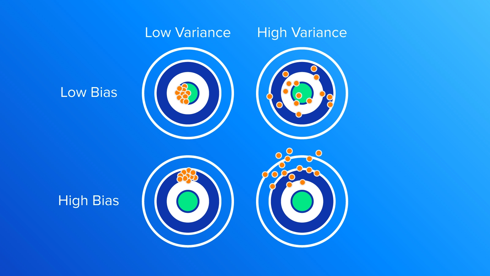
As shown in the above image, a high variance tends to disperse the model’s output, as the model is overly complex and fits the training data too closely. Essentially, the model captured the noise in the training data instead of the underlying patterns.
While in the case of high bias, the model tends to produce a similar output for almost all input values, which is far from the true relationship between the input and output. An optimum model complexity lies in the balance between these two errors, as we will see in the trade-off section, where the model has enough flexibility to capture the underlying patterns in the data but not so much that it overfits the noise or idiosyncrasies of the training data.
The bias-variance tradeoff refers to the balance that is needed between bias and variance to build a model that can generalize well to new data. A model that is too simple will have high bias but low variance, while a model that is too complex will have low bias but high variance. The goal is to find the right level of complexity that minimizes both bias and variance, resulting in a model that can accurately generalize to new data.
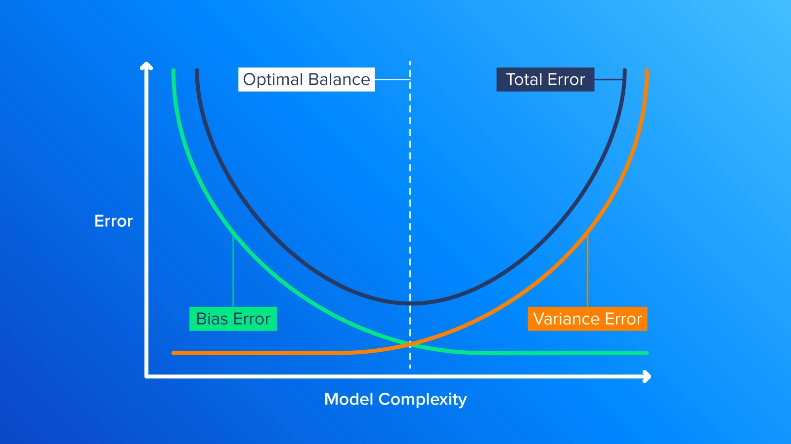
To strike a balance between bias and variance, we want to find the optimal level of model complexity that allows it to accurately predict the prices of the houses while also generalizing well to new data. This can be done by creating an error vs. model complexity graph, which shows the performance of the model at different levels of complexity. By analyzing this graph, we can identify the optimal level of model complexity where the bias and variance trade-off is balanced.
Developing your models on the cloud or on a local machine also sparks the need for balance. Leverage an Exxact Deep Learning System for lower TCO for your deep learning full-scale development and deployment.
Plotting a graph of error versus model complexity starts by building a series of models with varying levels of complexity. For instance, if we’re creating a linear regression model, we might begin with a simple model that has just one feature and gradually include more features to make the models more complex.
We would then train each model on a portion of our data and evaluate its performance on a separate test set. To measure the prediction error on the test set, we could use a metric like mean squared error (MSE) or mean absolute error (MAE).
After we have trained and evaluated each model, we can plot the test error against model complexity. The resulting graph typically shows a U-shaped curve, where error decreases as model complexity increases, reducing bias. However, the error eventually starts to increase again as the model becomes too complex and starts overfitting the data, which increases variance.
To determine the optimal complexity for bias and variance, look for the point on the graph where the test error is the lowest(as depicted by the dotted line in the middle of the graph). This point represents the optimal balance between bias and variance for this specific problem.
Generalization is the ability of a model to perform well on new data. A model that generalizes well is able to make accurate predictions on new data, which is important if we want to use the model in the real world. On the other hand, a model that doesn't generalize well may perform well on the data that it was trained on but may not make accurate predictions on new data. This is a problem because it means the model may not be useful in practice.
When we train a machine learning model, we want it to be able to make accurate predictions not just on the data that we use to train it but on new data that it has never seen before. This is because, in the real world, we don't always have access to the exact same data that we used to train the model but new first-time-seen data points. Therefore, it's important to train models that not only fit the training data well but also generalize well to new data.
Various regularization technique helps to prevent overfitting by adding a penalty term to the loss function, which discourages the model from becoming too complex.
There are two types of regularization that are commonly used: L1(Lasso) and L2(Ridge) regularization.
While all three approaches do add a penalty term to the loss function, in the case of Lasso regression, the regularization approach adds a penalty term to the loss function that is proportional to the absolute(modules) value of the model parameters.
This approach encourages the model to give less weight to unimportant features as it has the effect of driving some of the parameters to zero, which can help with feature selection. This means that it can help to identify which features are the most important and discard the rest. This can be really useful when working with high-dimensional datasets, where there are many features to choose from.
Lasso Regression can be particularly useful in high-dimensional datasets where the number of independent variables is much larger than the number of samples. In these cases, Lasso Regression can help to identify the most important variables and reduce the impact of noise.
Lasso Regression can be particularly useful in high-dimensional datasets where the number of independent variables is much larger than the number of samples. In these cases, Lasso Regression can help to identify the most important variables and reduce the impact of noise.
Ridge Regression is another type of linear regression that can be used to deal with overfitting in machine learning models. It's similar to Lasso Regression in that it adds a penalty term(regularization term) to the loss function, but instead of using the absolute value of the coefficients like Lasso Regression, it uses the square of the coefficients.
This has the effect of shrinking the coefficients of the less important variables towards zero, but unlike Lasso Regression, Ridge Regression doesn't set them exactly to zero. This means that Ridge Regression can't perform feature selection as well as Lasso Regression does, but it's better suited for cases where all the features are important to some degree.
Ridge Regression is particularly useful when dealing with datasets that have a high degree of collinearity (correlation between the features). In such cases, the model may have trouble determining which features are important and which are not, leading to overfitting. By adding a penalty term to the loss function, Ridge Regression can help to reduce overfitting and make the model more accurate.
Elastic Net Regression combines the best of both worlds by using techniques from both Ridge Regression and Lasso Regression. By adding both the Ridge Regression and Lasso Regression penalty terms to the loss function, Elastic Net Regression can perform both feature selection and feature shrinkage, which makes it more flexible and powerful than either technique alone.
The L1 regularization term tries to set some of the coefficients in the model to zero, which is useful for feature selection. This means it can identify the most important features that help to predict the target variable and exclude the less important features.
On the other hand, the L2 regularization term helps to control the magnitude of the coefficients in the model. This is useful for feature shrinkage, which means it reduces the impact of less important features on the model's performance.
Elastic Net Regression is particularly useful when working with datasets that have a large number of features and a high degree of multicollinearity, where the model may have difficulty distinguishing between important and unimportant features. By identifying and shrinking the less important features, Elastic Net Regression can help to reduce overfitting and improve the generalization performance of a model.
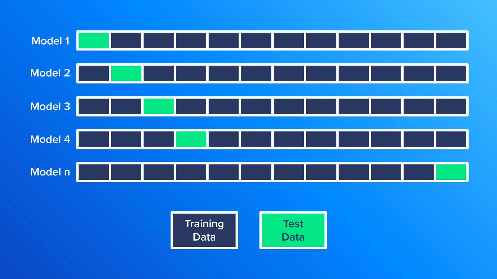
One popular cross-validation technique is k-fold cross-validation, where the data is divided into k equally sized parts. The model is trained on k-1 of the parts and tested on the remaining part. This process is repeated k times, with each part being used for testing once, and the performance is averaged across all iterations.
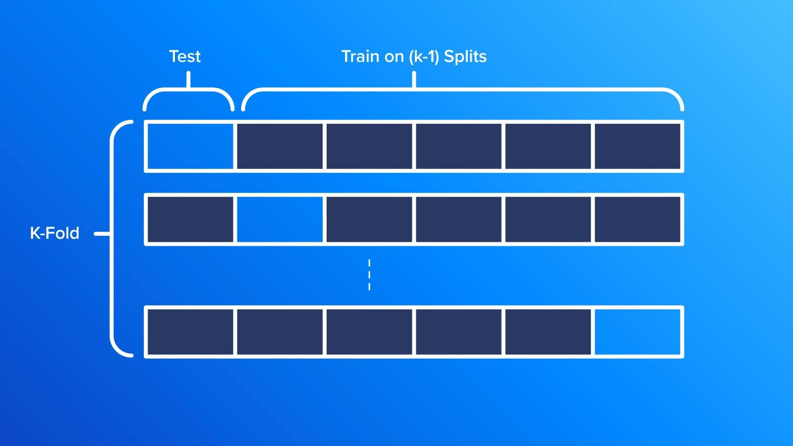
Leave-one-out cross-validation is another technique where a single data point is left out as the testing set, and the model is trained on the remaining data points. Note that the leave-one-out cross-validation is a special case of k-fold cross-validation, where k is equal to the number of data points in the dataset. For each iteration, a single data point is left out as the testing set, and the model is trained on the remaining data points. This process is repeated for each data point, and the average performance is computed.
Choosing the right complexity for a machine learning model is crucial to its performance. A model that's too simple won't capture the data's complexity and will underfit, while a model that's too complex will overfit the data and won't perform well on new data.
To choose the optimal model complexity, start with a simple model and gradually increase complexity until you get satisfactory results. Split the data into training, validation, and testing sets, and use the validation set to select the best model complexity. Use cross-validation to evaluate the model's performance on different data subsets.
Finally, use regularization techniques like L1, L2, and Elastic Net to prevent overfitting. The key is to balance model fit and complexity, evaluate performance, and prevent overfitting, so the model can generalize well to new data.
Exxact builds custom workstations, servers, and clusters to cater to your needs and requirements.
Contact us today for more information!
Machine learning is a complex field, with one of its biggest challenges is building models that can predict outcomes for new data. Building a model that fits the training data perfectly is easy, but the real test is whether it can accurately predict outcomes for new data.
This article delves into the concepts of overfitting and generalization and explores how they relate to the bias vs. variance trade-off. We will also discuss techniques for avoiding overfitting and finding the optimal balance between bias and variance in our models.
In machine learning, overfitting is a common problem that occurs when a model becomes too complex and starts to fit the training data too closely. This means that the model may not generalize well to new, unseen data because it has essentially memorized the training data instead of truly learning the underlying patterns or relationships. In technical terms, think about a regression model that requires a linear relationship, but instead is represented using a polynomial one.
Overfitting happens when the model is too good at learning from the training data but not so good at generalizing to new data. This can be a particular issue with deep learning models, which have many parameters that can be adjusted to fit the training data.
Underfitting is the opposite of overfitting in machine learning. In the case of underfitting (see leftmost graph above), we're essentially referring to a situation where the model is just too simple for the task at hand. In other words, the model doesn't have the necessary complexity to capture the underlying patterns in the data. In technical terms, think about a regression model that requires a polynomial equation, but instead is represented using a linear relationship.
Another way to think about underfitting is to consider the example of predicting housing prices. If we were to create a model that only takes into account the size of a house and ignores other important factors like the number of bedrooms, then this model might underfit the data. This occurs because the model is not taking into account all of the relevant information and thus is unable to accurately predict housing prices.
An underfit model tends to have high bias and low variance, which means that it makes a lot of errors in both the training and testing data. This is because the model is not able to capture the relationships between the data and is, therefore, unable to make accurate predictions.
The optimum model complexity is the sweet spot where the machine learning model is neither too simple nor too complex, but just right for the data it's working with. If a model is too simple, it may not capture all the important patterns and relationships in the data and can lead to underfitting. On the other hand, if the model is too complex, it may start to memorize the training data instead of learning the underlying patterns, which can lead to overfitting.
The goal of finding the optimum model complexity is to strike a balance between model fit and model complexity, where the model is simple enough to generalize well to new data but complex enough to capture the important patterns in the training data.
In the rest of this article, we will focus on different techniques that can be used to find the optimum model complexity, such as starting with a simple model and gradually increasing its complexity, cross-validation to evaluate the model on different subsets of the data, and using regularization techniques to prevent overfitting.
But first, let's start by explaining two very important concepts in machine learning, which are bias and variance.
Imagine trying to create a model to predict the price of a house based on its size. We have a dataset of 100 houses with their corresponding prices and sizes. To make predictions, we decide to use a linear regression model that only takes into account the size of the house.
Now, there are two problems that can occur when creating a model: bias and variance. Bias happens when the model is too simple and can't accurately capture the patterns in the data. In this case, if we use a linear model with only one feature (size), the model would likely not accurately predict the prices of the houses, leading to high bias.
On the other hand, variance occurs when the model is too complex and overfits the data, meaning it fits the training data too closely but doesn't perform well on new, unseen data. In this case, if we were to use a high-order polynomial model with many features (e.g. size squared, size cubed, etc.), it could overfit the data, resulting in high variance.
As shown in the above image, a high variance tends to disperse the model’s output, as the model is overly complex and fits the training data too closely. Essentially, the model captured the noise in the training data instead of the underlying patterns.
While in the case of high bias, the model tends to produce a similar output for almost all input values, which is far from the true relationship between the input and output. An optimum model complexity lies in the balance between these two errors, as we will see in the trade-off section, where the model has enough flexibility to capture the underlying patterns in the data but not so much that it overfits the noise or idiosyncrasies of the training data.
The bias-variance tradeoff refers to the balance that is needed between bias and variance to build a model that can generalize well to new data. A model that is too simple will have high bias but low variance, while a model that is too complex will have low bias but high variance. The goal is to find the right level of complexity that minimizes both bias and variance, resulting in a model that can accurately generalize to new data.
To strike a balance between bias and variance, we want to find the optimal level of model complexity that allows it to accurately predict the prices of the houses while also generalizing well to new data. This can be done by creating an error vs. model complexity graph, which shows the performance of the model at different levels of complexity. By analyzing this graph, we can identify the optimal level of model complexity where the bias and variance trade-off is balanced.
Developing your models on the cloud or on a local machine also sparks the need for balance. Leverage an Exxact Deep Learning System for lower TCO for your deep learning full-scale development and deployment.
Plotting a graph of error versus model complexity starts by building a series of models with varying levels of complexity. For instance, if we’re creating a linear regression model, we might begin with a simple model that has just one feature and gradually include more features to make the models more complex.
We would then train each model on a portion of our data and evaluate its performance on a separate test set. To measure the prediction error on the test set, we could use a metric like mean squared error (MSE) or mean absolute error (MAE).
After we have trained and evaluated each model, we can plot the test error against model complexity. The resulting graph typically shows a U-shaped curve, where error decreases as model complexity increases, reducing bias. However, the error eventually starts to increase again as the model becomes too complex and starts overfitting the data, which increases variance.
To determine the optimal complexity for bias and variance, look for the point on the graph where the test error is the lowest(as depicted by the dotted line in the middle of the graph). This point represents the optimal balance between bias and variance for this specific problem.
Generalization is the ability of a model to perform well on new data. A model that generalizes well is able to make accurate predictions on new data, which is important if we want to use the model in the real world. On the other hand, a model that doesn't generalize well may perform well on the data that it was trained on but may not make accurate predictions on new data. This is a problem because it means the model may not be useful in practice.
When we train a machine learning model, we want it to be able to make accurate predictions not just on the data that we use to train it but on new data that it has never seen before. This is because, in the real world, we don't always have access to the exact same data that we used to train the model but new first-time-seen data points. Therefore, it's important to train models that not only fit the training data well but also generalize well to new data.
Various regularization technique helps to prevent overfitting by adding a penalty term to the loss function, which discourages the model from becoming too complex.
There are two types of regularization that are commonly used: L1(Lasso) and L2(Ridge) regularization.
While all three approaches do add a penalty term to the loss function, in the case of Lasso regression, the regularization approach adds a penalty term to the loss function that is proportional to the absolute(modules) value of the model parameters.
This approach encourages the model to give less weight to unimportant features as it has the effect of driving some of the parameters to zero, which can help with feature selection. This means that it can help to identify which features are the most important and discard the rest. This can be really useful when working with high-dimensional datasets, where there are many features to choose from.
Lasso Regression can be particularly useful in high-dimensional datasets where the number of independent variables is much larger than the number of samples. In these cases, Lasso Regression can help to identify the most important variables and reduce the impact of noise.
Lasso Regression can be particularly useful in high-dimensional datasets where the number of independent variables is much larger than the number of samples. In these cases, Lasso Regression can help to identify the most important variables and reduce the impact of noise.
Ridge Regression is another type of linear regression that can be used to deal with overfitting in machine learning models. It's similar to Lasso Regression in that it adds a penalty term(regularization term) to the loss function, but instead of using the absolute value of the coefficients like Lasso Regression, it uses the square of the coefficients.
This has the effect of shrinking the coefficients of the less important variables towards zero, but unlike Lasso Regression, Ridge Regression doesn't set them exactly to zero. This means that Ridge Regression can't perform feature selection as well as Lasso Regression does, but it's better suited for cases where all the features are important to some degree.
Ridge Regression is particularly useful when dealing with datasets that have a high degree of collinearity (correlation between the features). In such cases, the model may have trouble determining which features are important and which are not, leading to overfitting. By adding a penalty term to the loss function, Ridge Regression can help to reduce overfitting and make the model more accurate.
Elastic Net Regression combines the best of both worlds by using techniques from both Ridge Regression and Lasso Regression. By adding both the Ridge Regression and Lasso Regression penalty terms to the loss function, Elastic Net Regression can perform both feature selection and feature shrinkage, which makes it more flexible and powerful than either technique alone.
The L1 regularization term tries to set some of the coefficients in the model to zero, which is useful for feature selection. This means it can identify the most important features that help to predict the target variable and exclude the less important features.
On the other hand, the L2 regularization term helps to control the magnitude of the coefficients in the model. This is useful for feature shrinkage, which means it reduces the impact of less important features on the model's performance.
Elastic Net Regression is particularly useful when working with datasets that have a large number of features and a high degree of multicollinearity, where the model may have difficulty distinguishing between important and unimportant features. By identifying and shrinking the less important features, Elastic Net Regression can help to reduce overfitting and improve the generalization performance of a model.
One popular cross-validation technique is k-fold cross-validation, where the data is divided into k equally sized parts. The model is trained on k-1 of the parts and tested on the remaining part. This process is repeated k times, with each part being used for testing once, and the performance is averaged across all iterations.
Leave-one-out cross-validation is another technique where a single data point is left out as the testing set, and the model is trained on the remaining data points. Note that the leave-one-out cross-validation is a special case of k-fold cross-validation, where k is equal to the number of data points in the dataset. For each iteration, a single data point is left out as the testing set, and the model is trained on the remaining data points. This process is repeated for each data point, and the average performance is computed.
Choosing the right complexity for a machine learning model is crucial to its performance. A model that's too simple won't capture the data's complexity and will underfit, while a model that's too complex will overfit the data and won't perform well on new data.
To choose the optimal model complexity, start with a simple model and gradually increase complexity until you get satisfactory results. Split the data into training, validation, and testing sets, and use the validation set to select the best model complexity. Use cross-validation to evaluate the model's performance on different data subsets.
Finally, use regularization techniques like L1, L2, and Elastic Net to prevent overfitting. The key is to balance model fit and complexity, evaluate performance, and prevent overfitting, so the model can generalize well to new data.
Exxact builds custom workstations, servers, and clusters to cater to your needs and requirements.
Contact us today for more information!
