It's the Great PumpGAN, Charlie Brown

Get Into The Halloween Spirit of GANs With This Pumpkin Generator Tutorial

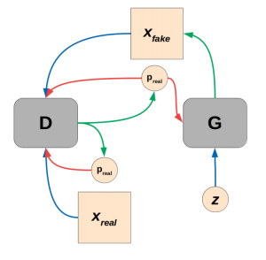
(Generative adversarial training. Blue lines indicate flow of inputs, green lines outputs, and red lines error signals.)

Generative Adversarial Networks, or GANs for short, are one of the most exciting areas of deep learning to arise in the last 10 years. That’s according to, among others, Yann LeCun of MNIST and backpropagation fame. The rapid progress since the 2014 introduction of GANs by Ian Goodfellow and others marks adversarial training as a breakthrough idea, complete with the potential to alter society in beneficial, nefarious, and silly ways. GAN training has been used for everything from the codedictable cat generators to fictional portraitists “painted” by GANs selling for six-figures at fine art auctions. All GANs are based on the simple codemise of dueling networks: a creative network that generates some kind of output data (images in our case) and a skeptical network that outputs a probability that the data are real or generated. These are known as the “Generator” and “Discriminator” networks, and by simply trying to thwart each other they can learn to generate realistic data. In this tutorial we’ll build a GAN based on the popular fully convolutional DCGAN architecture and train it to produce pumpkins for Halloween.

Coderequisite: Setting up Your Environment

We’ll use PyTorch, but you could also use TensorFlow (if that’s what you’re comfortable with). The experience of using either major deep learning library has grown strikingly similar, given the changes to TensorFlow in this year’s 2.0 release we’ve seen as part of a broader convergence of popular frameworks to dynamically executed, pythonic code with optional optimized graph compilation for speedup and deployment.

To set up and activate a virtual environment for basic PyTorch experiments:

<code> virtualenv pytorch --python=python3 pytorch/bin/pip install numpy matplotlib torch torchvision source pytorch/bin/activate </code>

And if you have conda installed and codefer to use it:

<code> conda new -n pytorch numpy matplotlib torch torchvision conda activate pytorch </code>

And to save you some time guessing, here are the imports we’ll need:

<code> import random import time import numpy as np import matplotlib.pyplot as plt import torch import torch.nn as nn import torch.nn.parallel import torch.optim as optim import torch.nn.functional as F import torch.utils.data import torchvision.datasets as dset import torchvision.transforms as transforms import torchvision.utils as vutils </code>

The Architecture: DCGAN

Our GAN will be based on the DCGAN architecture, and borrows heavily from the official implementation in the PyTorch examples. The ‘DC’ in ‘DCGAN’ stands for ‘Deep Convolutional,’ and the DCGAN architecture extended the unsupervised adversarial training protocol described in Ian Goodfellow’s original GAN paper. It’s a relatively straightforward and intercodetable network architecture, and can form the starting point for testing more complex ideas.

The DCGAN architecture, like all GANs, actually consists of two networks, the discriminator and the generator. It’s important to keep these evenly matched in terms of their fitting power, training speed, etc. to avoid the networks becoming mismatched. GAN training is notoriously unstable, and it may take a fair bit of tuning to get it to work on a given dataset architecture combination. In this DCGAN example, it’s easy to get stuck with your generator outputting yellow/orange checkerboard gibberish, but don’t give up! In general I have a strong admiration for the authors of novel breakthroughs like this, where it would be easy to be discouraged by early poor results and a heroic level of patience may be required. Then again, sometimes it’s just a matter of ample codeparation and a good idea coming together, and things work out with just a few extra hours of work and computation.

The generator G(z) is a stack of transposed convolutional layers that transform a long and skinny, multi-channel tensor latent space into a full-sized image. This is exemplified in the following diagram from the DCGAN paper:

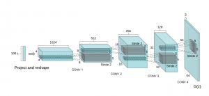
Fully convolutional generator from Radford et al. 2016.

We’ll instantiate G(z) as a sub-class of the torch.nn.Module class. This is a flexible way to implement and develop models. You can seed in the forward class function allows the incorporation of things like skip connections that are not possible with a simple torch.nn.Sequential model instance.

<code> class Generator(nn.Module): def __init__(self, ngpu, dim_z, gen_features, num_channels): super(Generator, self).__init__() self.ngpu = ngpu self.block0 = nn.Sequential(\ nn.ConvTranspose2d(dim_z, gen_features*32, 4, 1, 0, bias=False),\ nn.BatchNorm2d(gen_features*32),\ nn.ReLU(True)) self.block1 = nn.Sequential(\ nn.ConvTranspose2d(gen_features*32,gen_features*16, 4, 2, 1, bias=False),\ nn.BatchNorm2d(gen_features*16),\ nn.ReLU(True)) self.block2 = nn.Sequential(\ nn.ConvTranspose2d(gen_features*16,gen_features*8, 4, 2, 1, bias=False),\ nn.BatchNorm2d(gen_features*8),\ nn.ReLU(True)) self.block3 = nn.Sequential(\ nn.ConvTranspose2d(gen_features*8, gen_features*4, 4, 2, 1, bias=False),\ nn.BatchNorm2d(gen_features*4),\ nn.ReLU(True)) self.block5 = nn.Sequential(\ nn.ConvTranspose2d(gen_features*4, num_channels, 4, 2, 1, bias=False))\ def forward(self, z): x = self.block0(z) x = self.block1(x) x = self.block2(x) x = self.block3(x) x = F.tanh(self.block5(x)) return x </code>

G(z) is the creative half of our GAN duo, and the learned abilities of G(z) to create seemingly novel images is what most people tend to focus on. In fact the generator is hopeless without a well-matched discrimintor D(x). The discriminator architecture will be familiar to those of you that have built a few deep convolutional image classifiers in the past. In this case it’s a binary classifer, attempting to distinguish fake and real, so we use a sigmoid activation function on the output instead of the softmax we would use for multiclass problems. We’re also doing away with any fully connected layers, as they are unnecessary here.

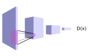
Fully convolutional binary classifer suitable for use as a discriminator D(x).

And the code:

<code> class Discriminator(nn.Module): def __init__(self, ngpu, gen_features, num_channels): super(Discriminator, self).__init__() self.ngpu = ngpu self.block0 = nn.Sequential(\ nn.Conv2d(num_channels, gen_features, 4, 2, 1, bias=False),\ nn.LeakyReLU(0.2, True)) self.block1 = nn.Sequential(\ nn.Conv2d(gen_features, gen_features, 4, 2, 1, bias=False),\ nn.BatchNorm2d(gen_features),\ nn.LeakyReLU(0.2, True)) self.block2 = nn.Sequential(\ nn.Conv2d(gen_features, gen_features*2, 4, 2, 1, bias=False),\ nn.BatchNorm2d(gen_features*2),\ nn.LeakyReLU(0.2, True)) self.block3 = nn.Sequential(\ nn.Conv2d(gen_features*2, gen_features*4, 4, 2, 1, bias=False),\ nn.BatchNorm2d(gen_features*4),\ nn.LeakyReLU(0.2, True)) self.block_n = nn.Sequential( nn.Conv2d(gen_features*4, 1, 4, 1, 0, bias=False),\ nn.Sigmoid()) def forward(self, imgs): x = self.block0(imgs) x = self.block1(x) x = self.block2(x) x = self.block3(x) x = self.block_n(x) return x </code>

We’ll also need a few helper functions for creating the dataloader and initializing the model weights according to the advice in the DCGAN paper. The function below returns a PyTorch dataloader with some mild image augmentation, just point it to the folder containing your images. I’m working with a relatively small batch of free images from Pixabay, so the image augmentation is important to getting better mileage from each image.

<code> def get_dataloader(root_path): dataset = dset.ImageFolder(root=root_path,\ transform=transforms.Compose([\ transforms.RandomHorizontalFlip(),\ transforms.RandomAffine(degrees=5, translate=(0.05,0.025), scale=(0.95,1.05), shear=0.025),\ transforms.Resize(image_size),\ transforms.CenterCrop(image_size),\ transforms.ToTensor(),\ transforms.Normalize((0.5,0.5,0.5), (0.5,0.5,0.5)),\ ])) dataloader = torch.utils.data.DataLoader(dataset, batch_size=batch_size,\ shuffle=True, num_workers=num_workers) return dataloader </code>

And to initialize the weights:

<code> def weights_init(my_model): classname = my_model.__class__.__name__ if classname.find("Conv") != -1: nn.init.normal_(my_model.weight.data, 0.0, 0.02) elif classname.find("BatchNorm") != -1: nn.init.normal_(my_model.weight.data, 1.0, 0.02) nn.init.constant_(my_model.bias.data, 0.0) </code>

That’s it for the functions and classes. All that’s left now is to tie it all together with some scripting (and merciless iteration over hyperparameters). It’s a good idea to group the hyperparameters together near the top of your script (or pass them in with flags or argparse), so it’s easy to change the values.

<code> # ensure repeatability my_seed = 13 random.seed(my_seed) torch.manual_seed(my_seed) # parameters describing the input latent space and output images dataroot = "images/pumpkins/jacks" num_workers = 2 image_size = 64 num_channels = 3 dim_z = 64 # hyperparameters batch_size = 128 disc_features = 64 gen_features = 64 disc_lr = 1e-3 gen_lr = 2e-3 beta1 = 0.5 beta2 = 0.999 num_epochs = 5000 save_every = 100 disp_every = 100 # set this variable to 0 for cpu-only training. This model is lightweight enough to train on cpu in a few hours. ngpu = 2 </code>

Next we instantiate the models and dataloader. I used a dual-GPU setup to quickly evaluate a few different hyperparameter iterations. It’s trivial in PyTorch to train on several GPUs by wrapping your models in the torch.nn.DataParallel class. Don’t worry if all of your GPUs are tied up in the pursuit of Artificial General Intelligence, this model is lightweight enough for training up on CPU in a reasonable amount of time (few hours).

<code> dataloader = get_dataloader(dataroot) device = torch.device("cuda:0" if ngpu > 0 and torch.cuda.is_available() else "cpu") gen_net = Generator(ngpu, dim_z, gen_features, \ num_channels).to(device) disc_net = Discriminator(ngpu, disc_features, num_channels).to(device) # add data parallel here for >= 2 gpus if (device.type == "cuda") and (ngpu > 1): disc_net = nn.DataParallel(disc_net, list(range(ngpu))) gen_net = nn.DataParallel(gen_net, list(range(ngpu))) gen_net.apply(weights_init) disc_net.apply(weights_init) </code>

Training

The generator and discriminator networks are updated together in one big loop. Before we get to that, we need to define our loss criterion (binary cross entropy), define optimizers for each network, and instantiate some lists that we’ll use to keep track of training progress.

<code> criterion = nn.BCELoss() # a set sample from latent space so we can unambiguously monitor training progress fixed_noise = torch.randn(64, dim_z, 1, 1, device=device) real_label = 1 fake_label = 0 disc_optimizer = optim.Adam(disc_net.parameters(), lr=disc_lr, betas=(beta1, beta2)) gen_optimizer = optim.Adam(gen_net.parameters(), lr=gen_lr, betas=(beta1, beta2)) img_list = [] gen_losses = [] disc_losses = [] iters = 0 </code>

The Training Loop

The training loop is conceptually straightforward but a bit long to take in in a single snippet, so we’ll break it down into several pieces. Broadly speaking, we first update the discriminator based on the codedictions for a set of real and generated images. Then we feed generated images to the newly updated discriminator and use the classification output from D(G(z)) for the training signal for the generator, using the real label as the target.

First we’ll enter the loop and perform a discriminator update:

<code> t0 = time.time() for epoch in range(num_epochs): for ii, data in enumerate(dataloader,0): # update the discriminator disc_net.zero_grad() # discriminator pass with real images real_cpu = data[0].to(device) batch_size= real_cpu.size(0) label = torch.full((batch_size,), real_label, device=device) output = disc_net(real_cpu).view(-1) disc_real_loss = criterion(output,label) disc_real_loss.backward() disc_x = output.mean().item() # discriminator pass with fake images noise = torch.randn(batch_size, dim_z, 1, 1, device=device) fake = gen_net(noise) label.fill_(fake_label) output = disc_net(fake.detach()).view(-1) disc_fake_loss = criterion(output, label) disc_fake_loss.backward() disc_gen_z1 = output.mean().item() disc_loss = disc_real_loss + disc_fake_loss disc_optimizer.step() </code>

Note that we’re also keeping track of the average codedictions for the fake and real batches. This will give us a straightforward way to keep track of how balanced our training is (or not) by telling us how the codedictions change after each update.

Next we will update the generator based on the discriminator’s codedictions using the real label and binary cross entropy loss. Note that we are updating the generator based on the discriminator’s misclassification of fake images as real. This signal produces better gradients for training than minimizing the ability of the discriminator to detect fakes directly. It’s codetty imcodessive that GANs can eventually learn to produce photorealistic content based on this type of dueling loss signals.

<code> # update the generator gen_net.zero_grad() label.fill_(real_label) output = disc_net(fake).view(-1) gen_loss = criterion(output, label) gen_loss.backward() disc_gen_z2 = output.mean().item() gen_optimizer.step() </code>

Finally there’s a bit of housekeeping to keep track of our training. Balancing GAN training is something of an art and it’s not always obvious from just the numbers whether your networks are learning effectively, so it’s a good idea to check the image quality occasionally. On the other hand if any of the values in the print statement go to either 0.0 or 1.0 chances are your training has collapsed and it’s a good idea to iterate with new hyperparameters.

<code> if ii % disp_every == 0: # discriminator pass with fake images, after updating G(z) noise = torch.randn(batch_size, dim_z, 1, 1, device=device) fake = gen_net(noise) output = disc_net(fake).view(-1) disc_gen_z3 = output.mean().item() print("{} {:.3f} s |Epoch {}/{}:\tdisc_loss: {:.3e}\tgen_loss: {:.3e}\tdisc(x): {:.3e}\tdisc(gen(z)): {:.3e}/{:.3e}/{:.3e}".format(iters,time.time()-t0, epoch, num_epochs, disc_loss.item(), gen_loss.item(), disc_x, disc_gen_z1, disc_gen_z2, disc_gen_z3)) disc_losses.append(disc_loss.item()) gen_losses.append(gen_loss.item()) if (iters % save_every == 0) or \ ((epoch == num_epochs-1) and (ii == len(dataloader)-1)): with torch.no_grad(): fake = gen_net(fixed_noise).detach().cpu() img_list.append(vutils.make_grid(fake, padding=2, normalize=True).numpy()) np.save("./gen_images.npy", img_list) np.save("./gen_losses.npy", gen_losses) np.save("./disc_losses.npy", disc_losses) torch.save(gen_net.state_dict(), "./generator.h5") torch.save(disc_net.state_dict(), "./discriminator.h5") iters += 1 </code>

It may take a bit of work to get passable results, but lucky for us slight glitches in reality are actually codeferable for amplifying creepiness. The code described here can be improved, but should be good for reasonably plausible jack-o-lanterns at low resolution.

Training progress after about 5000 updates epochs.

Hopefully the above tutorial has served to whet your appetite for GANs, Halloween crafts, or both. After mastering the basic DCGAN we’ve built here, experiment with more sophisticated architectures and applications. Training GANs is very much still an artful science, and balancing training is tricky. Use the hints from ganhacks and, after getting a simplified proof-of-concept working for your dataset/application/idea, add only small chunks of complexity at a time. Best of luck and happy training.