Atrous Convolutions & U-Net Architectures for Deep Learning: A Brief History

A Turning Point for Deep Learning

Every once in a while a new tool is developed that is so much more effective than what was previously available that it spreads through people and their endeavors like a flood, permanently altering the landscape that came before.

Deep learning is one of those tools.

We often point to the 2012 ImageNet competition as the day the dam broke. In a dataset with millions of images arranged in thousands of categories, the convolutional neural network previously known as "SuperVision" (aka AlexNet) achieved a top-5 error rate of just over 15%.

The next closest competitor achieved a relatively unimpressive error rate around 25%, comparable to the models that had won in previous years. A similar breakthrough in recognizing handwritten digits took place in the late 1990s with Yann LeCun and Yoshua Bengio's LeNet architecture.

From the 90s to Modern Times - Neural Network Developments

The difference between 1990s neural networks mastering handwritten digit recognition (such as the famous 10-class MNIST dataset and the human-level image classification nets we have today largely comes down to improved deep learning software and hardware tools for effective hardware use. The basic network architecture, multiple layers connected by convolution operations, and the training algorithm, back-propagation of error gradients, remain largely the same.

Convolutions, the butter to the bread in conv-nets, involve sliding windowed clusters of weights known as kernels across an input image. At each position, multiplying the kernel weights with the local pixels produces a neural activation on the next layer. By stacking multiple convolutional layers the network learns to extract increasingly abstract features.

Deep Learning - Applications Move from Cat Identification to Solving Real World Issues

Although you might be forgiven for thinking the main purpose of deep learning is identifying cats in images and videos, in fact deep learning can be adapted to perform myriad visual and inferential tasks, outperforming the previously state of the art for tasks as diverse as localized image captioning, super-resolution, and perspective synthesis.

For example, biomedical imaging historically relies on expert analysis in both clinical and research settings. On the clinical side of things, X-rays, MRIs, and pathology sections are increasingly being diagnosed with the aid of deep learning. In research, partially automated microscopy experiments may generate terabytes of data from a single experiment, and the individual cells and cell components in these images have to be both segmented and classified, known in machine learning parlance as "semantic segmentation." Even with the best conventional computer vision algorithms, the bottleneck in these experiments often comes down to human curation of mis-segmented images.

This is an important enough topic to have formed the basis for the 2018 Data Science Bowl, a competition put on by Kaggle, Booz Allen Hamilton, and the Broad Institute to improve the state of the art in generalized cell nucleus segmentation.

Variations on fully convolutional neural networks, also known as end-to-end deep learning, are particularly well suited for these kinds of image processing tasks.

Learned Feature Engineering / Deep Learning Conv-Nets

A key element of deep learning’s ascension to prominence has been learned feature engineering: stacked convolution operations extract appropriate features by minimizing the error for the task at hand via back-propagation. That is to say, human expertise and manual effort fine-tuning feature extraction is replaced by an algorithm implementing the chain rule of calculus. Where previously a computer vision task could have been accomplished by a bespoke combination of hand-engineered features (with such appealing names as HOG, SIFT, and GLOH), a deep learning conv-net explores an error-gradient landscape to automatically learn a set of network weights for extracting relevant features for the task at hand.

It is often the case that deep conv-nets work almost too well.

Compared to a conventional computer vision algorithm, it’s relatively easy to get reasonably good performance without much effort and without fully understanding how and why a conv-net is getting results. When researchers come up with a new model architecture, we can expect them to put most of their effort into proving it works well instead of trying to determine why it works or challenging the model in a way that might make it look unfavorable.

Personally replicating and investigating methods that claim to work a certain way pays dividends in understanding what conv-net variants might best apply to a given scenario.

Semantic Segmentation: Translation Invariance vs. Translation Equivariance

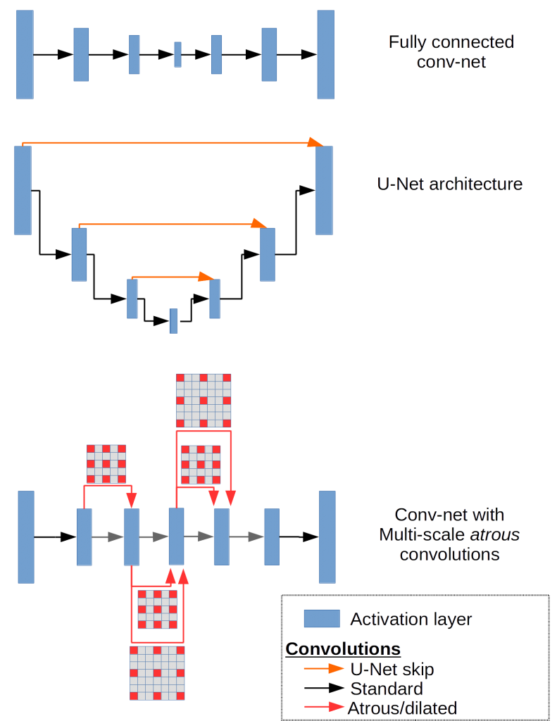
One way that conv-nets achieve what’s known as translation invariance - the ability to recognize an object regardless of where it appears in an image - is by sequentially reducing the image dimensions in both x and y dimensions (pooling) while increasing the depth (e.g. by increasing the number of convolutional kernels).

Applied sequentially in deep nets, this is one reason that conv-nets perform so well at image classification.

But for semantic segmentation we don’t want translation invariance but rather translation equivariance: we want a model to be able to recognize the object regardless of its location but also to be able to pinpoint the location of the object. Consider that a conv-net with 3 pooling layers, such as AlexNet, will reduce the x,y dimensionality of the input image by 8x, and modern conv-nets are generally much deeper. Although we can design a conv-net to learn how to upsample these representations with transposed convolutions, semantic segmentation still often underperforms in the fine details.

For semantic segmentation in research microscopy the most important data may correspond to abnormal or tightly clustered morphology of cell nuclei (hallmarks of cancer progression).

Conv-Net Improvements: Dilated Convolutions (Atrous Convolutions) and U-Net architectures

Several improvements to fully connected conv-nets for semantic segmentation of fine details have been (re)investigated in the last few years.

Dilated convolutions or atrous convolutions, previously described for wavelet analysis without signal decimation, expands window size without increasing the number of weights by inserting zero-values into convolution kernels.

In the deep learning framework TensorFlow, atrous convolutions are implemented with function:

tf.nn.atrous_conv2d

Models written in Theano can likewise use the argument

filter_dilation

to:

theano.tensor.nnet.conv2d

to implement atrous convolutions.

Dilated convolutions have been shown to decrease blurring in semantic segmentation maps, and are purported to work at least in part by extracting long range information without the need for pooling.

Using U-Net architectures is another method that seeks to retain high spatial frequency information by directly adding skip connections between early and late layers. To investigate how well these techniques stack up, we’ll train three networks based on a simple fully-connected conv-net, a conv-net invoking multi-scale convolutions using atrous convolutions, and a conv-net with skip connections in the style of U-Net.

These are relatively shallow 8 layer networks each constrained to have the same total number of weights, and we train them on a dataset of 400 672x512 fluorescence images of cell nuclei (data from Coelho et al. 2009).

To see what kinds of features each conv-net is capable of extracting, we can train them as autoencoders, an unsupervised technique for learning efficient data representations by reconstructing the input image at the output. This is a simple method for determining what parts of the input a network is capable of representing internally by what appears at the output.

Take for example, these test images (not included in training or validation) reconstructed by a fully-connected conv-net:

The insensitivity to fine details is evident in the reconstructions, blurring out bright spots and boundaries between adjacent cell nuclei. The most likely explanation for those bright spots are heterochromatin foci, where DNA is stored in tightly bound packets when genes are not expressed. It’s reasonable to envision an experiment that involves segmenting and classifying a mixed population of cells with high and low prevalence of heterochromatin foci, indicating abnormal gene expression associated with disease or mutation.

Can we improve on the resolution of these foci and boundary resolution with the techniques mentioned above?

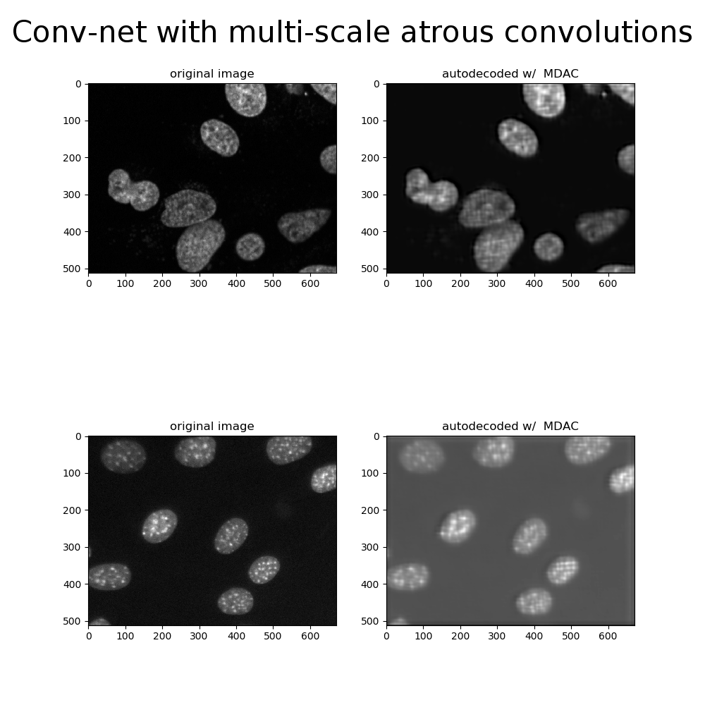
In fact, we can get improved multi-scale reconstructions using atrous convolutions. By dilating convolution kernels with empty weights the network learns long-distance features without relying on pooling functions, and without pooling the network can retain more of high spatial-frequency details.

Thanks to the dilated holes in convolution kernels, using atrous convolutions doesn’t require training any more weights than the fully-connected conv-net. However, the network still must keep layer activations in memory during training and inference, and decreased pooling operations mean the size of these activation tensors will be much larger. This limits the size of the input images we can test on and gives us less options for trying out different batch sizes.

Ultimately, this will reduce the total depth we can achieve on given hardware depending on how much memory is available on the GPU, and will usually train more slowly to boot. Perhaps using a U-Net architecture can give us the best of both worlds: improved retention of fine detail features with fast training of deep networks.

U-Net Architecture, Multi-Scale Conv-Net with Atrous Convolutions: Advantages & Drawbacks

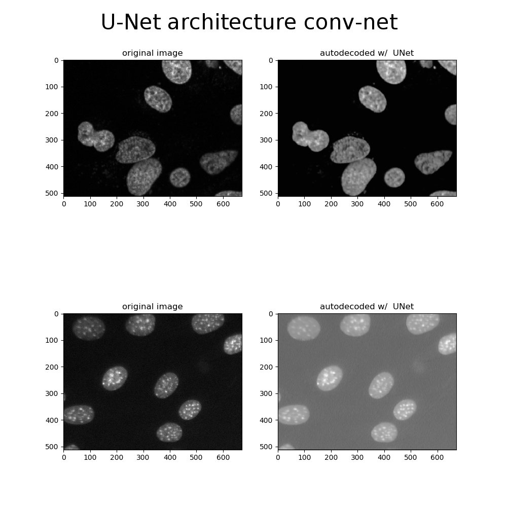
Indeed, the test results from the U-Net architecture are qualitatively better than either the fully-connected and the multi-scale conv-net with atrous convolutions. The only obvious drawback to U-Net style architectures is that learning may slow down in the middle layers of deeper models, so there is some risk of the network learning to ignore the layers where abstract features are represented. This is due to gradients becoming diluted further away from the output of a network, where the error is computed, resulting in slower learning for far-removed weights.

The advantages of U-Net models are probably worth the risk, though, and choosing the right activation functions and regularization parameters can probably mitigate adverse effects caused by vanishing gradients in the middle layers of U-Net models, but those are topics for another time.

In practice we may want to combine atrous convolutions and U-Net architectures for further improvements for multi-scale vision tasks, achieving better performance than either method alone, but the simple comparison above tells us the U-Nets find it much easier to learn fine details than other architectures, albeit with some risks to be aware of.

Deep learning works so well that it is easy and tempting to throw together seemingly arbitrary model architectures or to copy the most recent techniques without taking the time to understand how they work.

On the other hand, investigating model variants in a controlled manner while devoting equal effort to optimizing or breaking each model in informative ways is essential if we are to make informed engineering decisions about model architectures. This doesn’t just apply to biomedical imaging, where recognizing fine details of heterochromatin foci or neuronal synapses might be important. In an industrial setting detecting a small-scale defect, designing illumination, orientation, and component sparsity to match the custom feature engineering of conventional computer vision algorithm may require many person-hours of effort. Alternatively a conv-net that achieves proper equivariance while retaining details can learn to distinguish these features automatically.