
Approaching the Problem of Equivariance with Hinton's Capsule Networks
Have a look at this:
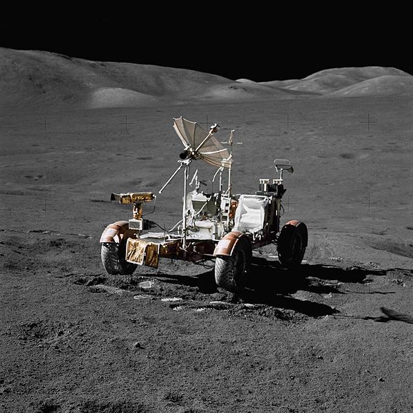
Now see this:
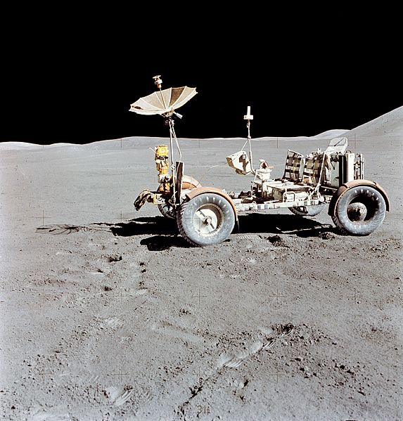
Even if you've never been to the moon, you can probably recognize the subject of the images above as NASA's Lunar Roving Vehicle, or at least as being two instances of an identical vehicle at slightly different orientations. You probably have an intuitive idea of how you could manipulate the viewpoint of one image to approximate the view of the other. This sort of cognitive transformation is effortlessly intuitive for a human, but turns out to be very difficult for a convolutional neural network without explicit training examples.
Limitations of Convolutional and Max Pooling Layers
Standard convolutional neural networks are made up of, as the name suggests, a series of convolution operations that hierarchically extract image features like edges, points, and corners. Each convolution multiplies the image by a sliding window of pixel weights, aka a convolution kernel, and there may be tens to thousands of kernels in each layer. Often, we perform a pooling operation in between each convolution, decreasing image dimensions. Pooling not only decreases the size of the layers (saving memory), but provides some translation invariance so that a given network can classify an image subject regardless of where it resides in the image. This may be more of a bug than a feature, however, as pooling operations confuse information about where something is in an image (driving the development of skip connections in U-nets) and fare poorly coping with image transformations other than translation.
Translation invariance in conv-nets with pooling falls short of object transformation equivariance, a more generalized cognitive ability that seems to be closer to our own approach to making sense of the world. The fact that conv-nets perform pretty well at a wide variety of computer vision tasks glosses over this shortcoming. Consider the classic example of the MNIST hand-written digits dataset. LeNet-5, a relatively shallow and simple conv-net design by today's standards, quickly learns to correctly identify 98% of the digits in the test dataset.

Test predicted: seven two one zero four one four nine
Test groundTruth: seven two one zero four one four nine
Accuracy of the network on the 10000 test images: 98.68 %
Apply a simple 35 degree rotation to the test images, however, and the test performance drops precipitously.

Test predicted: four two one zero four one four two
Test groundTruth: seven two one zero four one four nine
LeNet 5 accuracy on 10000 (rotated) test images: 76.05 %
A so-called "Capsule Network" does somewhat better with rotated data:
Test predicted: nine zero one two three four five six
Test groundTruth: seven two one zero four one four nine
Accuracy of the network on the 10000 (rotated) test images: 84.09 %
The standard approach to mitigate the problem is data augmentation, that is, adding rotations, mirroring, distortion, etc. to synthetically enlarge the dataset to cover a larger distribution of possible examples. This improves performance on a given vision task, but it's clearly a kludge, and, as they say "intellectually unsatisfying."
For many years Geoffrey Hinton has been outspoken in his dislike for pooling operations, and has been trying to replace the happenstance translational invariance of pooling with a more universal equivariance with what he terms "capsules," a representation of scene contents created by reshaping the features extracted by convolution into multidimensional vectors. The concept of capsule networks has evolved alongside the upsurge in conv-nets as transforming autoencoders (2011) to a dynamic routing method for training capsules (2017), and most recently with an updated training algorithm termed expectation maximalization (2018).
Capsules to the Rescue?
In capsule networks, each vector learns to represent some aspect of the image, such as shape primitives, with vector length corresponding to the probability of the object existing at a given point, and the direction of the vector describing the object's characteristics. In the 2017 implementation, the first layer of capsules each try to predict the correct probabilities for the next layer of capsules via dynamic routing (e.g. in a face detection CapsNet the "eye" and "nose" capsule values will each contribute to the prediction of the "face" capsule in the next layer for each point). Consider the simplified example of 2D capsule vectors detecting polygons that make up cartoon doorways. These capsules represent the presence and orientation of two shapes, blocks and quarter circles, and together they will try to predict the correct classification in the next capsule layer, which learns to detect a properly oriented doorway.
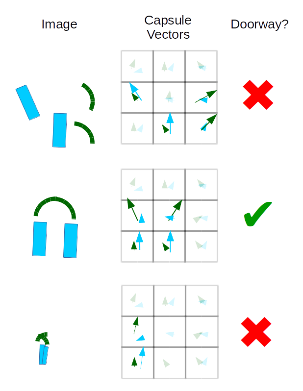
Whereas in a conv-net the mere presence of the correct features (in orientations that are represented in the training data) is enough to trigger a classification regardless of their spatial relationship to one another, capsule vectors all have to be in strong agreement to predict the whole from its parts. We should also take note that a capsule can only detect one instance of a given object at a time, so a pile of blocks would be indistinguishable and CapsNet models can get confused by overlapping parts of the same type. This shortcoming is often compared to crowding in human perception.
Tutorial Section: Training and Testing LeNet5 vs. Dynamic Routing CapsNet for Rotated MNIST Classification
Even better than talking about capsules is tinkering with them. To keep things simple, we'll be working with the popular MNIST handwritten digits dataset. The code in this section provides a hackable foundation for understanding CapsNets in the context of a familiar dataset and machine learning model in the 5-layer LeNet5 conv-net. After getting a general overview of CapsNet performance on MNIST, we'd recommend adding different training data augmentation routines to see how well each model takes to learning various transformations.
First we'll define the dataset we want to work with and the preprocessing we need, using PyTorch's transform library.
import torch
import torchvision
import torchvision.transforms as transforms
import numpy as np
import matplotlib.pyplot as plt
import time

import torch.nn as nn
import torch.nn.functional as F
import torch.optim as optim

#Download dataset (if necessary) and define test set transformation

batch_size = 8
degrees= 15

transform_normal = transforms.Compose([torchvision.transforms.RandomAffine(0, translate=(0.0714,0.0714)),\
transforms.ToTensor(),\
transforms.Normalize((0.5, 0.5, 0.5), (0.5, 0.5, 0.5))])

transform_rotate = transforms.Compose([torchvision.transforms.RandomRotation([degrees,degrees+1e-7],\
resample=False,\
expand=False, center=None),\
transforms.ToTensor(),\
transforms.Normalize((0.5, 0.5, 0.5), (0.5, 0.5, 0.5))])

train = torchvision.datasets.MNIST(root='./data', train=True,download=True,transform=transform_normal)
test = torchvision.datasets.MNIST(root='./data', train=False,download=True,transform=transform_rotate)
test_norot = torchvision.datasets.MNIST(root='./data', train=False,download=True,transform=transform_normal)

#Data iterator definitions
train_loader = torch.utils.data.DataLoader(train, batch_size=batch_size,shuffle=True)
test_loader = torch.utils.data.DataLoader(test, batch_size=batch_size,shuffle=False)
test_loader_norot = torch.utils.data.DataLoader(test_norot, batch_size=batch_size,shuffle=False)

#Define class labels
classes = ("zero", "one", "two", "three", "four", "five", "six", "seven", "eight", "nine", "ten")
Defining our CNN: LeNet5
We'll start by implementing a small convolutional neural network called LeNet5 in PyTorch. This model gives us test set accuracy in the high 90s after only a few training epochs, and consists of just 2 convolutional and 3 fully connected layers.
#define LeNet5 Conv-net architecture

class lenet5(nn.Module):
def __init__(self):
super(lenet5, self).__init__()

in_channels = 1
conv0_channels = 6
conv1_channels = 16
kernel_size = 5
pool_size = 2
pool_stride = 2

h_in = 256
h2 = 120
h3 = 84
classes = 10

self.conv0 = nn.Conv2d(in_channels, conv0_channels, kernel_size)
self.pool = nn.AvgPool2d(pool_size, pool_stride)
self.conv1 = nn.Conv2d(conv0_channels, conv1_channels, kernel_size)
self.fc2 = nn.Linear(h_in, h2)
self.fc3 = nn.Linear(h2, h3)
self.fc4 = nn.Linear(h3, classes)

def forward(self, x):
h_in = 256
x = self.pool(F.relu(self.conv0(x)))
x = self.pool(F.relu(self.conv1(x)))
x = x.view(-1, h_in)
x = F.relu(self.fc2(x))
x = F.relu(self.fc3(x))
x = self.fc4(x)
return x

def imshow(img,my_string=None):
#Helper function for visualizing digits
img = img / 2 + 0.5 # unnormalize
npimg = img.numpy()
plt.imshow(np.transpose(npimg, (1, 2, 0)))
if(my_string is not None):
plt.title(my_string)
plt.show()
Training and Test Routines for LeNet5
We'll use Adam optimization to minimize cross-entropy error during training. Again, this functionality is readily accessible via PyTorch.
def train_lenet5(lenet5,learning_rate=1e-4, epochs=10, try_cuda=True):

t0 = time.time()

if (try_cuda):
if torch.cuda.is_available():
device = torch.device("cuda")
else:
device = torch.device("cpu")

#Define training criterion and optimizer
criterion = nn.CrossEntropyLoss()
optimizer = optim.Adam(lenet5.parameters(), lr=learning_rate)

#Send model to GPU if desired
lenet5 = lenet5.to(device)

for epoch in range(epochs): # loop over the dataset multiple times

running_loss = 0.0
for i, data in enumerate(train_loader, 0):

#get inputs
inputs, labels = data
inputs = inputs.to(device)
labels = labels.to(device)

#zero the parameter gradients
optimizer.zero_grad()

#forward pass + back-propagation + update parameters
outputs = lenet5(inputs)
loss = criterion(outputs, labels)
loss.backward()
optimizer.step()

#print statistics
running_loss += loss.item()
if i % 2000 == 1999: # print every 2000 mini-batches
print('[%d, %5d] loss: %.3f' %
(epoch + 1, i + 1, running_loss / 2000))
running_loss = 0.0

print("Finished training for %i epochs on device %s took %.2f seconds"%(epochs,device,time.time()-t0))

def test_lenet5(lenet5):
#We'll test on the cpu
lenet5.to(torch.device("cpu"))
#Get training set performance
dataiter = iter(train_loader)
images, labels = dataiter.next()

#print images
imshow(torchvision.utils.make_grid(images),"Training Example")

pred_prob = lenet5(images)
_, predicted = torch.max(pred_prob, 1)

#report labels
print('Predicted: ', ' '.join('%5s' % classes[predicted[j]] for j in range(batch_size)))
print('GroundTruth: ', ' '.join('%5s' % classes[labels[j]] for j in range(batch_size)))

#calculate accuracy
correct = 0
total = 0
with torch.no_grad():
for data in test_loader_norot:
images, labels = data
outputs = lenet5(images)
_, predicted = torch.max(outputs.data, 1)
total += labels.size(0)
correct += (predicted == labels).sum().item()

print("LeNet 5 accuracy on (unrotated) training images: %.2f %%" % (100 * correct / total))

dataiter = iter(test_loader_norot)
images, labels = dataiter.next()

#print images
imshow(torchvision.utils.make_grid(images),"Unrotated Test Data")

#get probabilities and predictions
pred_prob = lenet5(images)
_, predicted = torch.max(pred_prob, 1)

print('Test predicted: ', ' '.join('%5s' % classes[predicted[j]] for j in range(batch_size)))
print('Test groundTruth: ', ' '.join('%5s' % classes[labels[j]] for j in range(batch_size)))

correct = 0
total = 0
with torch.no_grad():
for data in test_loader_norot:
images, labels = data
outputs = lenet5(images)
_, predicted = torch.max(outputs.data, 1)
total += labels.size(0)
correct += (predicted == labels).sum().item()

print("LeNet 5 accuracy on 10000 (unrotated) test images: %.2f %%" % (100 * correct / total))

#test with rotation
dataiter = iter(test_loader)
images, labels = dataiter.next()

#print images
imshow(torchvision.utils.make_grid(images),"Rotated Test Data")

pred_prob = lenet5(images)

_, predicted = torch.max(pred_prob, 1)

print("Test predicted: ", " ".join("%5s" % classes[predicted[j]] for j in range(batch_size)))
print("Test groundTruth: ", " ".join("%5s" % classes[labels[j]] for j in range(batch_size)))

correct = 0
total = 0
with torch.no_grad():
for data in test_loader:
images, labels = data
outputs = lenet5(images)
_, predicted = torch.max(outputs.data, 1)
total += labels.size(0)
correct += (predicted == labels).sum().item()

print("LeNet 5 accuracy on 10000 (rotated) test images: %.2f %%" % (100 * correct / total))

lenet5_model = lenet5()

pre_trained = True # Change this flag to train from scratch
if(pre_trained):
lenet5_model.load_state_dict(torch.load("./lenet5_trained.pt"))
else:
#liy: learn-it-yourself
pass
print("LeNet5 Parameters: \n",lenet5)

train_lenet5(lenet5_model,epochs=1)
test_lenet5(lenet5_model)

#save the model parameters
#torch.save(lenet5_model.state_dict(), "./lenet5_trained.pt")
#output [1, 2000] loss: 1.135 [1, 4000] loss: 0.521 ... [14, 6000] loss: 0.051
The dynamic routing algorithm for training capsule networks is more computationally demanding than for conv-nets. We'll definitely want to train on a GPU if we want to finish in a reasonable amount of time. We've also pre-trained a CapsNet for those who find themselves between GPUs at the moment or just want to skip to testing. For training and testing a capsule network, we forked and modified the implementation at https://github.com/gram-ai/capsule-networks by Kenta Iwasaki. Clone the version used in this tutorial by entering (in the command line):
git clone https://github.com/theScinder/capsule_networks_rotated_MNIST.git
After that, you'll probably want to spin up a PyTorch visdom server for visualization purposes by entering (in a separate command line window):
python -m visdom.server
Finally, you can train and test the CapsNet by entering the code below into an interactive python session (still in the capsule_networks_rotated_MNIST directory), or save it as a .py to play around with and run it from the command line with:
python run_capsnet.py
where run_capsnet.py is the name of the newly saved script file.
from capsule_network import * from torch.autograd import Variable #change these parameters to train from scratch num_epochs = 0 load_model = True train_and_test_capsnet()
#output #parameters: 8215570 WARNING:root:Setting up a new session... time to train CapsNet for 0 epochs = 0.04 seconds Test predicted: seven two one zero four one four nine Test groundTruth: seven two one zero four one four nine Accuracy of the network on the 10000 (unrotated) test images: 99.37 % Test predicted: nine zero one two three four five six Test groundTruth: seven two one zero four one four nine Accuracy of the network on the 10000 (rotated) test images: 92.12 %
Conclusions
Capsule Networks provide an extension of the universal feature extraction properties of convolutional neural networks. By training each primary capsule to predict the output of the next layer's capsules, the model can be encouraged to learn to recognize the relationships between parts, wholes, and the importance of their instantiation characteristics such as location and orientation. In many ways this feels like a more natural way to recognize the objects in a scene, as orientations and other attributes can be learned as parameters of a scene object represented by the capsules, and modifying the characteristics can give us realistic changes in viewpoint, scale, etc. Convolution activations start to seem like a pretty crude level of feature representation by comparison.
The dynamic routing algorithm used for training can be painfully slow (one epoch can take over five minutes vs 25 seconds for LeNet5 on same hardware), however, and in practice it can take a bit of selective representation (aka cherry-picking) to find situations where CapsNets are decidedly better than a comparable conv-net. Data augmentation can yield greater than 98% accuracy across training and (rotated) test MNIST datasets with a simple conv-net like LeNet5, and it may be more fair to compare CapsNets to conv-nets based on training time required rather than model size. Overall, the difference between 98% and upper 99% accuracy may not seem like much, but it's those last few percentage points of error that matter most in terms of solving a problem rather than learning an approximate heuristic.
There's still plenty of room for improvements to training CapsNets, and the high level of interest ensures that they will receive plenty of development effort. We'll probably see CapsNets gain utility in a similar way that conv-nets did, first being demonstrated on toy problems like MNIST before application to more relevant domains. One thing that's sure to yield exciting results with CapsNets is a combination of faster hardware accelerators and better training algorithms/software libraries to allow "Deep CapsNets" to become practical.
Images of the Lunar Roving Vehicle in the public domain (generated by NASA)
The PyTorch implementation of a dynamic routing CapsNet was forked and modified from a public repository by Kenta Iwasaki @ Gram.AI: https://github.com/gram-ai/capsule-networks

Approaching the Problem of Equivariance with Hinton's Capsule Networks
Approaching the Problem of Equivariance with Hinton's Capsule Networks
Have a look at this:

Now see this:

Even if you've never been to the moon, you can probably recognize the subject of the images above as NASA's Lunar Roving Vehicle, or at least as being two instances of an identical vehicle at slightly different orientations. You probably have an intuitive idea of how you could manipulate the viewpoint of one image to approximate the view of the other. This sort of cognitive transformation is effortlessly intuitive for a human, but turns out to be very difficult for a convolutional neural network without explicit training examples.
Limitations of Convolutional and Max Pooling Layers
Standard convolutional neural networks are made up of, as the name suggests, a series of convolution operations that hierarchically extract image features like edges, points, and corners. Each convolution multiplies the image by a sliding window of pixel weights, aka a convolution kernel, and there may be tens to thousands of kernels in each layer. Often, we perform a pooling operation in between each convolution, decreasing image dimensions. Pooling not only decreases the size of the layers (saving memory), but provides some translation invariance so that a given network can classify an image subject regardless of where it resides in the image. This may be more of a bug than a feature, however, as pooling operations confuse information about where something is in an image (driving the development of skip connections in U-nets) and fare poorly coping with image transformations other than translation.
Translation invariance in conv-nets with pooling falls short of object transformation equivariance, a more generalized cognitive ability that seems to be closer to our own approach to making sense of the world. The fact that conv-nets perform pretty well at a wide variety of computer vision tasks glosses over this shortcoming. Consider the classic example of the MNIST hand-written digits dataset. LeNet-5, a relatively shallow and simple conv-net design by today's standards, quickly learns to correctly identify 98% of the digits in the test dataset.

Test predicted: seven two one zero four one four nine
Test groundTruth: seven two one zero four one four nine
Accuracy of the network on the 10000 test images: 98.68 %
Apply a simple 35 degree rotation to the test images, however, and the test performance drops precipitously.

Test predicted: four two one zero four one four two
Test groundTruth: seven two one zero four one four nine
LeNet 5 accuracy on 10000 (rotated) test images: 76.05 %
A so-called "Capsule Network" does somewhat better with rotated data:
Test predicted: nine zero one two three four five six
Test groundTruth: seven two one zero four one four nine
Accuracy of the network on the 10000 (rotated) test images: 84.09 %
The standard approach to mitigate the problem is data augmentation, that is, adding rotations, mirroring, distortion, etc. to synthetically enlarge the dataset to cover a larger distribution of possible examples. This improves performance on a given vision task, but it's clearly a kludge, and, as they say "intellectually unsatisfying."
For many years Geoffrey Hinton has been outspoken in his dislike for pooling operations, and has been trying to replace the happenstance translational invariance of pooling with a more universal equivariance with what he terms "capsules," a representation of scene contents created by reshaping the features extracted by convolution into multidimensional vectors. The concept of capsule networks has evolved alongside the upsurge in conv-nets as transforming autoencoders (2011) to a dynamic routing method for training capsules (2017), and most recently with an updated training algorithm termed expectation maximalization (2018).
Capsules to the Rescue?
In capsule networks, each vector learns to represent some aspect of the image, such as shape primitives, with vector length corresponding to the probability of the object existing at a given point, and the direction of the vector describing the object's characteristics. In the 2017 implementation, the first layer of capsules each try to predict the correct probabilities for the next layer of capsules via dynamic routing (e.g. in a face detection CapsNet the "eye" and "nose" capsule values will each contribute to the prediction of the "face" capsule in the next layer for each point). Consider the simplified example of 2D capsule vectors detecting polygons that make up cartoon doorways. These capsules represent the presence and orientation of two shapes, blocks and quarter circles, and together they will try to predict the correct classification in the next capsule layer, which learns to detect a properly oriented doorway.

Whereas in a conv-net the mere presence of the correct features (in orientations that are represented in the training data) is enough to trigger a classification regardless of their spatial relationship to one another, capsule vectors all have to be in strong agreement to predict the whole from its parts. We should also take note that a capsule can only detect one instance of a given object at a time, so a pile of blocks would be indistinguishable and CapsNet models can get confused by overlapping parts of the same type. This shortcoming is often compared to crowding in human perception.
Tutorial Section: Training and Testing LeNet5 vs. Dynamic Routing CapsNet for Rotated MNIST Classification
Even better than talking about capsules is tinkering with them. To keep things simple, we'll be working with the popular MNIST handwritten digits dataset. The code in this section provides a hackable foundation for understanding CapsNets in the context of a familiar dataset and machine learning model in the 5-layer LeNet5 conv-net. After getting a general overview of CapsNet performance on MNIST, we'd recommend adding different training data augmentation routines to see how well each model takes to learning various transformations.
First we'll define the dataset we want to work with and the preprocessing we need, using PyTorch's transform library.
import torch
import torchvision
import torchvision.transforms as transforms
import numpy as np
import matplotlib.pyplot as plt
import time

import torch.nn as nn
import torch.nn.functional as F
import torch.optim as optim

#Download dataset (if necessary) and define test set transformation

batch_size = 8
degrees= 15

transform_normal = transforms.Compose([torchvision.transforms.RandomAffine(0, translate=(0.0714,0.0714)),\
transforms.ToTensor(),\
transforms.Normalize((0.5, 0.5, 0.5), (0.5, 0.5, 0.5))])

transform_rotate = transforms.Compose([torchvision.transforms.RandomRotation([degrees,degrees+1e-7],\
resample=False,\
expand=False, center=None),\
transforms.ToTensor(),\
transforms.Normalize((0.5, 0.5, 0.5), (0.5, 0.5, 0.5))])

train = torchvision.datasets.MNIST(root='./data', train=True,download=True,transform=transform_normal)
test = torchvision.datasets.MNIST(root='./data', train=False,download=True,transform=transform_rotate)
test_norot = torchvision.datasets.MNIST(root='./data', train=False,download=True,transform=transform_normal)

#Data iterator definitions
train_loader = torch.utils.data.DataLoader(train, batch_size=batch_size,shuffle=True)
test_loader = torch.utils.data.DataLoader(test, batch_size=batch_size,shuffle=False)
test_loader_norot = torch.utils.data.DataLoader(test_norot, batch_size=batch_size,shuffle=False)

#Define class labels
classes = ("zero", "one", "two", "three", "four", "five", "six", "seven", "eight", "nine", "ten")
Defining our CNN: LeNet5
We'll start by implementing a small convolutional neural network called LeNet5 in PyTorch. This model gives us test set accuracy in the high 90s after only a few training epochs, and consists of just 2 convolutional and 3 fully connected layers.
#define LeNet5 Conv-net architecture

class lenet5(nn.Module):
def __init__(self):
super(lenet5, self).__init__()

in_channels = 1
conv0_channels = 6
conv1_channels = 16
kernel_size = 5
pool_size = 2
pool_stride = 2

h_in = 256
h2 = 120
h3 = 84
classes = 10

self.conv0 = nn.Conv2d(in_channels, conv0_channels, kernel_size)
self.pool = nn.AvgPool2d(pool_size, pool_stride)
self.conv1 = nn.Conv2d(conv0_channels, conv1_channels, kernel_size)
self.fc2 = nn.Linear(h_in, h2)
self.fc3 = nn.Linear(h2, h3)
self.fc4 = nn.Linear(h3, classes)

def forward(self, x):
h_in = 256
x = self.pool(F.relu(self.conv0(x)))
x = self.pool(F.relu(self.conv1(x)))
x = x.view(-1, h_in)
x = F.relu(self.fc2(x))
x = F.relu(self.fc3(x))
x = self.fc4(x)
return x

def imshow(img,my_string=None):
#Helper function for visualizing digits
img = img / 2 + 0.5 # unnormalize
npimg = img.numpy()
plt.imshow(np.transpose(npimg, (1, 2, 0)))
if(my_string is not None):
plt.title(my_string)
plt.show()
Training and Test Routines for LeNet5
We'll use Adam optimization to minimize cross-entropy error during training. Again, this functionality is readily accessible via PyTorch.
def train_lenet5(lenet5,learning_rate=1e-4, epochs=10, try_cuda=True):

t0 = time.time()

if (try_cuda):
if torch.cuda.is_available():
device = torch.device("cuda")
else:
device = torch.device("cpu")

#Define training criterion and optimizer
criterion = nn.CrossEntropyLoss()
optimizer = optim.Adam(lenet5.parameters(), lr=learning_rate)

#Send model to GPU if desired
lenet5 = lenet5.to(device)

for epoch in range(epochs): # loop over the dataset multiple times

running_loss = 0.0
for i, data in enumerate(train_loader, 0):

#get inputs
inputs, labels = data
inputs = inputs.to(device)
labels = labels.to(device)

#zero the parameter gradients
optimizer.zero_grad()

#forward pass + back-propagation + update parameters
outputs = lenet5(inputs)
loss = criterion(outputs, labels)
loss.backward()
optimizer.step()

#print statistics
running_loss += loss.item()
if i % 2000 == 1999: # print every 2000 mini-batches
print('[%d, %5d] loss: %.3f' %
(epoch + 1, i + 1, running_loss / 2000))
running_loss = 0.0

print("Finished training for %i epochs on device %s took %.2f seconds"%(epochs,device,time.time()-t0))

def test_lenet5(lenet5):
#We'll test on the cpu
lenet5.to(torch.device("cpu"))
#Get training set performance
dataiter = iter(train_loader)
images, labels = dataiter.next()

#print images
imshow(torchvision.utils.make_grid(images),"Training Example")

pred_prob = lenet5(images)
_, predicted = torch.max(pred_prob, 1)

#report labels
print('Predicted: ', ' '.join('%5s' % classes[predicted[j]] for j in range(batch_size)))
print('GroundTruth: ', ' '.join('%5s' % classes[labels[j]] for j in range(batch_size)))

#calculate accuracy
correct = 0
total = 0
with torch.no_grad():
for data in test_loader_norot:
images, labels = data
outputs = lenet5(images)
_, predicted = torch.max(outputs.data, 1)
total += labels.size(0)
correct += (predicted == labels).sum().item()

print("LeNet 5 accuracy on (unrotated) training images: %.2f %%" % (100 * correct / total))

dataiter = iter(test_loader_norot)
images, labels = dataiter.next()

#print images
imshow(torchvision.utils.make_grid(images),"Unrotated Test Data")

#get probabilities and predictions
pred_prob = lenet5(images)
_, predicted = torch.max(pred_prob, 1)

print('Test predicted: ', ' '.join('%5s' % classes[predicted[j]] for j in range(batch_size)))
print('Test groundTruth: ', ' '.join('%5s' % classes[labels[j]] for j in range(batch_size)))

correct = 0
total = 0
with torch.no_grad():
for data in test_loader_norot:
images, labels = data
outputs = lenet5(images)
_, predicted = torch.max(outputs.data, 1)
total += labels.size(0)
correct += (predicted == labels).sum().item()

print("LeNet 5 accuracy on 10000 (unrotated) test images: %.2f %%" % (100 * correct / total))

#test with rotation
dataiter = iter(test_loader)
images, labels = dataiter.next()

#print images
imshow(torchvision.utils.make_grid(images),"Rotated Test Data")

pred_prob = lenet5(images)

_, predicted = torch.max(pred_prob, 1)

print("Test predicted: ", " ".join("%5s" % classes[predicted[j]] for j in range(batch_size)))
print("Test groundTruth: ", " ".join("%5s" % classes[labels[j]] for j in range(batch_size)))

correct = 0
total = 0
with torch.no_grad():
for data in test_loader:
images, labels = data
outputs = lenet5(images)
_, predicted = torch.max(outputs.data, 1)
total += labels.size(0)
correct += (predicted == labels).sum().item()

print("LeNet 5 accuracy on 10000 (rotated) test images: %.2f %%" % (100 * correct / total))

lenet5_model = lenet5()

pre_trained = True # Change this flag to train from scratch
if(pre_trained):
lenet5_model.load_state_dict(torch.load("./lenet5_trained.pt"))
else:
#liy: learn-it-yourself
pass
print("LeNet5 Parameters: \n",lenet5)

train_lenet5(lenet5_model,epochs=1)
test_lenet5(lenet5_model)

#save the model parameters
#torch.save(lenet5_model.state_dict(), "./lenet5_trained.pt")
#output [1, 2000] loss: 1.135 [1, 4000] loss: 0.521 ... [14, 6000] loss: 0.051
The dynamic routing algorithm for training capsule networks is more computationally demanding than for conv-nets. We'll definitely want to train on a GPU if we want to finish in a reasonable amount of time. We've also pre-trained a CapsNet for those who find themselves between GPUs at the moment or just want to skip to testing. For training and testing a capsule network, we forked and modified the implementation at https://github.com/gram-ai/capsule-networks by Kenta Iwasaki. Clone the version used in this tutorial by entering (in the command line):
git clone https://github.com/theScinder/capsule_networks_rotated_MNIST.git
After that, you'll probably want to spin up a PyTorch visdom server for visualization purposes by entering (in a separate command line window):
python -m visdom.server
Finally, you can train and test the CapsNet by entering the code below into an interactive python session (still in the capsule_networks_rotated_MNIST directory), or save it as a .py to play around with and run it from the command line with:
python run_capsnet.py
where run_capsnet.py is the name of the newly saved script file.
from capsule_network import * from torch.autograd import Variable #change these parameters to train from scratch num_epochs = 0 load_model = True train_and_test_capsnet()
#output #parameters: 8215570 WARNING:root:Setting up a new session... time to train CapsNet for 0 epochs = 0.04 seconds Test predicted: seven two one zero four one four nine Test groundTruth: seven two one zero four one four nine Accuracy of the network on the 10000 (unrotated) test images: 99.37 % Test predicted: nine zero one two three four five six Test groundTruth: seven two one zero four one four nine Accuracy of the network on the 10000 (rotated) test images: 92.12 %
Conclusions
Capsule Networks provide an extension of the universal feature extraction properties of convolutional neural networks. By training each primary capsule to predict the output of the next layer's capsules, the model can be encouraged to learn to recognize the relationships between parts, wholes, and the importance of their instantiation characteristics such as location and orientation. In many ways this feels like a more natural way to recognize the objects in a scene, as orientations and other attributes can be learned as parameters of a scene object represented by the capsules, and modifying the characteristics can give us realistic changes in viewpoint, scale, etc. Convolution activations start to seem like a pretty crude level of feature representation by comparison.
The dynamic routing algorithm used for training can be painfully slow (one epoch can take over five minutes vs 25 seconds for LeNet5 on same hardware), however, and in practice it can take a bit of selective representation (aka cherry-picking) to find situations where CapsNets are decidedly better than a comparable conv-net. Data augmentation can yield greater than 98% accuracy across training and (rotated) test MNIST datasets with a simple conv-net like LeNet5, and it may be more fair to compare CapsNets to conv-nets based on training time required rather than model size. Overall, the difference between 98% and upper 99% accuracy may not seem like much, but it's those last few percentage points of error that matter most in terms of solving a problem rather than learning an approximate heuristic.
There's still plenty of room for improvements to training CapsNets, and the high level of interest ensures that they will receive plenty of development effort. We'll probably see CapsNets gain utility in a similar way that conv-nets did, first being demonstrated on toy problems like MNIST before application to more relevant domains. One thing that's sure to yield exciting results with CapsNets is a combination of faster hardware accelerators and better training algorithms/software libraries to allow "Deep CapsNets" to become practical.
Images of the Lunar Roving Vehicle in the public domain (generated by NASA)
The PyTorch implementation of a dynamic routing CapsNet was forked and modified from a public repository by Kenta Iwasaki @ Gram.AI: https://github.com/gram-ai/capsule-networks


