Artificial Intelligence
NVIDIA RAPIDS Tutorial: GPU Accelerated Data Processing
January 6, 2022
13 min read

.jpg?format=webp)
What even is RAPIDS? The short answer: RAPIDS allows data scientists to execute high-performance data science tasks with the help of GPU acceleration.
While the use of GPUs and distributed computing is widely discussed in the academic and business circles for core AI/ML tasks (e.g. running a 100-layer deep neural network for image classification or billion-parameter BERT speech synthesis model), they find less coverage when it comes to their utility for regular data science and data engineering tasks. These data-related tasks are the essential precursor to any ML workload in an AI pipeline and they often constitute a majority percentage of the time and intellectual effort spent by a data scientist or even an ML engineer.
So, the important question is: Can we leverage the power of GPU and distributed computing for regular data processing jobs too?
RAPIDS is a very good answer to that question.
It is a suite of open-source software libraries and APIs that gives you the ability to execute end-to-end data science and analytics pipelines entirely on GPUs. NVIDIA incubated this project and built tools to take advantage of CUDA primitives for low-level compute optimization. It specifically focuses on exposing GPU parallelism and high-bandwidth memory speed features through the friendly Python language popular with all the data scientists and analytics professionals.
Common data preparation and wrangling tasks are highly valued in the RAPIDS ecosystem. It also lends a significant amount of support for multi-node, multi-GPU deployment, and distributed processing. Wherever possible, it integrates with other libraries which make out-of-memory (i.e. dataset size larger than individual computer RAM) data processing easy and accessible for individual data scientists.
Interested in a workstation for data science research?
Accelerate your data science development with an Exxact solution starting at $5,500
Here are the main components of this ecosystem,
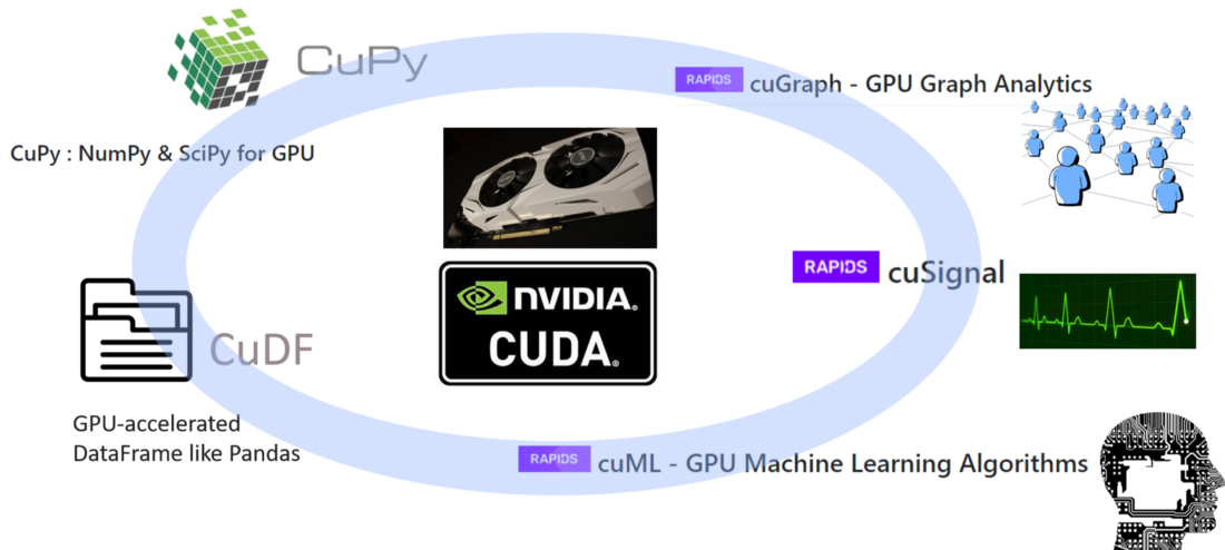
Image source: GPU-Powered Data Science (NOT Deep Learning) with RAPIDS
The three most prominent (and Pythonic) components, that are of particular interest to common data scientists, are as follows.
A CUDA-powered array library that looks and feels just like Numpy, while using various CUDA libraries e.g., cuBLAS, cuDNN, cuRand, cuSolver, cuSPARSE, cuFFT, and NCCL to take full advantage of the GPU architecture underneath.
This is a GPU DataFrame library for loading, aggregating, joining, filtering, and manipulating data with a pandas-like API. Data engineers and data scientists can use it to easily accelerate their task flows using powerful GPUs without ever learning the nuts and bolts of CUDA programming.
This library enables data scientists, analysts, and researchers to run traditional/classical ML algorithms and associated processing tasks fully leveraging the power of a GPU. Naturally, this is used mostly with tabular datasets. Think about Scikit-learn and what it could do with all those hundreds of Cuda and Tensor Cores on your GPU card! On cue to that, in most cases, cuML’s Python API matches that of Scikit-learn. Furthermore, it tries to offer multi-GPU and multi-node-GPU support by integrating gracefully with Dask, wherever it can, for taking advantage of true distributed processing/cluster computing.
In this short tutorial, we will show some canonical code examples from these libraries and compare them with similar code from standard Python libraries.
Setup with Saturn Cloud
The latest version of RAPIDS needs the following:
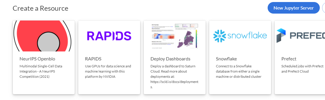
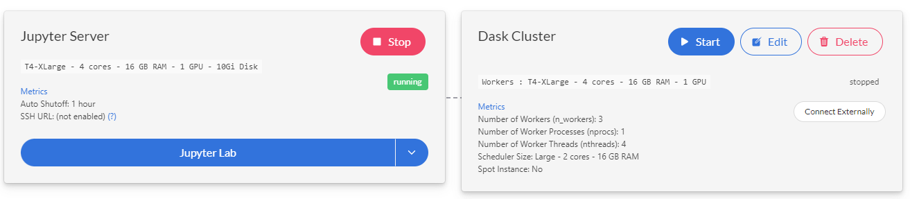
You can do a local install, or you can use Google Colab or any other Cloud GPU hosting service. For this tutorial, we used the Saturn Cloud platform. You can choose a RAPIDS deployment right from the homepage of your Saturn Cloud account.
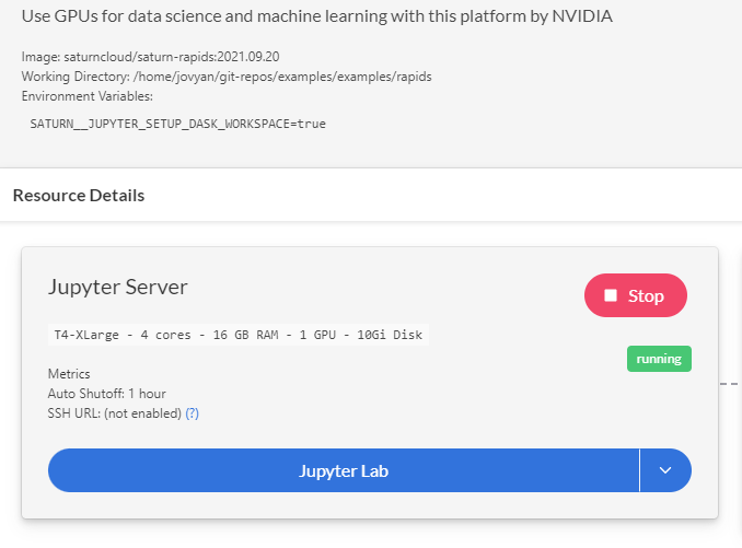
On the next page, you have to start a Jupyter server to launch a Jupyter notebook:
Start by importing both Numpy and CuPy and other supporting libraries for the code.
import numpy as np, cupy as cp
import matplotlib.pyplot as plt
from tqdm import tqdm
import time
Define arrays
You can define arrays just like Numpy:
a1 = cp.array([1,2,3])
a2 = cp.arange(1,11,2)
a3 = cp.random.normal(size=(3,3))
When we print these arrays, they look just as expected:
a1
>> array([1, 2, 3])

a2
>> array([1, 3, 5, 7, 9])

a3
>> array([[-0.05483573,  0.51381329, -0.2292121 ],
       [ 1.01891233,  0.84549515, -0.22683239],
       [-0.24651295,  1.03496478, -0.11075805]])
The type is CuPy.
type(a1)
>> cupy._core.core.ndarray
Standard Numpy ops
All the standard Numpy operations are supported. Examples are shown below.
Transpose
a3.T
>> array([[-0.05483573,  1.01891233, -0.24651295],
       [ 0.51381329,  0.84549515,  1.03496478],
       [-0.2292121 , -0.22683239, -0.11075805]])
Adding a scalar
a3+1
>> array([[0.94516427, 1.51381329, 0.7707879 ],
       [2.01891233, 1.84549515, 0.77316761],
       [0.75348705, 2.03496478, 0.88924195]])
Mean along a particular axis (‘0’ for row and ‘1’ for column in case of two dimensions)
a3.mean(axis=1)
>> array([0.07658849, 0.54585836, 0.22589793])
A simple Boolean filtering to keep only positive numbers in the two-dimensional array
a3*(a3>0)
>> array([[-0.        ,  0.51381329, -0.        ],
       [ 1.01891233,  0.84549515, -0.        ],
       [-0.        ,  1.03496478, -0.        ]])
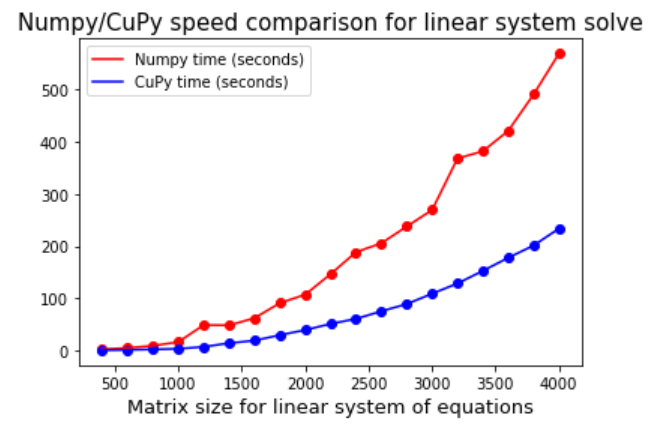
A linear algebra op speed comparison with Numpy
Finally, we show a true Numpy-like usage and how the RAPIDS compare to Numpy in terms of performance. We solve a linear system of equations using the linalg.solve routine for various sizes of matrices and compare the speed of solution.
Here is the code to do the calculation and save the timing with Numpy only:
size=[200*i for i in range(1,21)]

numpy_time = []
for s in tqdm(size):
    a = np.array([np.random.randint(-10,10,s).tolist() for i in range(s)])
    b = np.array([np.random.randint(-100,100,s)]).T
    t1 = time.time()
    x = np.linalg.solve(a,b)
    t2 = time.time()
    delta_t = (t2-t1)*1000
    numpy_time.append(delta_t)
Now, the great thing with RAPIDS is that, in most cases, we need minimal code change to take advantage of the library because of API similarity. Therefore, the above code needs just the replacement of a single word in a few places to take advantage of GPU acceleration. We just replaced numpy with cupy and np with cp.
cupy_time = []
for s in tqdm(size):
    a = cp.array([np.random.randint(-10,10,s).tolist() for i in range(s)])
    b = cp.array([np.random.randint(-100,100,s)]).T
    t1 = time.time()
    x = cp.linalg.solve(a,b)
    t2 = time.time()
    delta_t = (t2-t1)*1000
    cupy_time.append(delta_t)
We can plot the comparative result with the following code and the result is shown subsequently.
plt.title("Numpy/CuPy speed comparison for linear system solve",fontsize=15)
plt.scatter(size[1:],numpy_time[1:],color='red',marker='o')
plt.plot(size[1:],numpy_time[1:],color='red')
plt.scatter(size[1:],cupy_time[1:],color='blue',
         marker='o')
plt.plot(size[1:],cupy_time[1:],color='blue')
plt.legend(['Numpy time (seconds)','CuPy time (seconds)'])
plt.xlabel("Matrix size for linear system of equations",fontsize=13)
plt.show()
We show some code examples with CuDF library using a dataset on US colleges. We read the dataset from Github and ingest it using the cudf.read_csv function just like we would do with Python Pandas.
import cudf
import io, requests
from io import StringIO

url = "https://raw.githubusercontent.com/tirthajyoti/Machine-Learning-with-Python/master/Datasets/College_Data"

content = requests.get(url).content.decode('utf-8')
cdf = cudf.read_csv(StringIO(content))
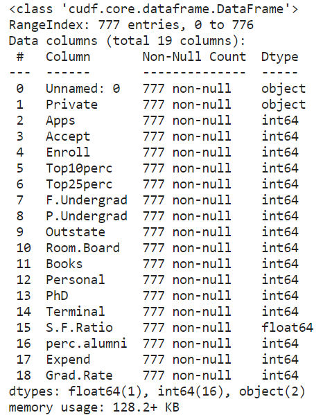
The type is CuDF as expected:
type(cdf)
>> cudf.core.dataframe.DataFrame
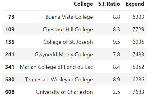
We can check the first few entries and the information just like in Pandas. The result is often truncated on the right side due to space limitations not showing all the columns.
cdf.head()
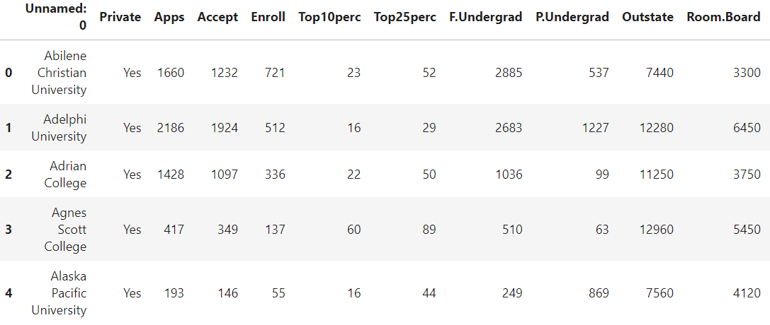
cdf.info()
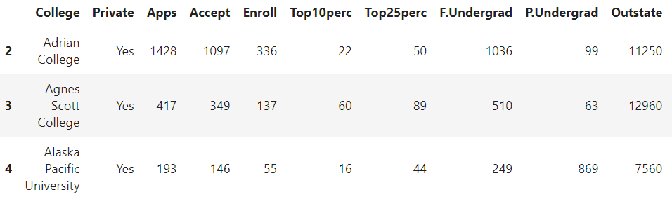
We can do regular indexing and filtering like we do with Pandas. Before that, we can rename the first column,
cdf.rename(columns={"Unnamed: 0": "College"},inplace=True)
Then, indexing,
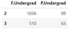
cdf.loc[2:4]
cdf[['F.Undergrad','P.Undergrad']][2:4]
Suppose we want to find colleges with low student-to-faculty ratio and also low expenditure. The filtering code works just like pandas:
filter_1 = cdf['S.F.Ratio']< 10
filter_2 = cdf['Expend'] < 8000
cdf[filter_1 & filter_2 ][['College','S.F.Ratio','Expend']]
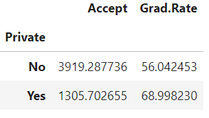
Group By Operations
We can do fast grouping operations with GPU acceleration. For example, if we wanted to group the college acceptance numbers and graduation rates by their ‘Private’ status, and take the average, we could do that in one line:
cdf.groupby('Private').mean()[['Accept','Grad.Rate']]
Getting Numpy arrays out of CuDF series
We have to remember a peculiarity of the CuDF (or CuPy for that matter) objects. They don't yield Numpy arrays by default and we need to add a .get() method at the end of the usual code to get the Numpy array for further processing. This is particularly important for visualizations, where we may need such Numpy arrays and cannot plot from CuPy or CuDF directly.
For example, if we want to plot the histogram of the number of PhD’s, we have to extract like this:
phds=cdf['PhD'].values.get()
So, we attached the .get() at the end of the usual .values method. Then, we can plot:
plt.title('Histogram of PhD',fontsize=15)
plt.hist(phds,edgecolor='k')
plt.show()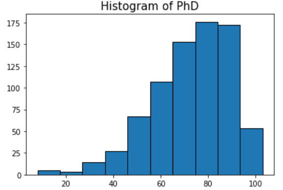
Distributed computing with Dask often goes hand in hand with RAPIDS using GPU clusters. The following code is an example of doing that mixing Dask and CuML together.
# Initialize UCX for high-speed transport of CUDA arrays
from dask_cuda import LocalCUDACluster

# Create a Dask single-node CUDA cluster w/ one worker per device
cluster = LocalCUDACluster(protocol="ucx",
                           enable_tcp_over_ucx=True,
                           enable_nvlink=True,
                           enable_infiniband=False)

from dask.distributed import Client
client = Client(cluster)

# Read CSV file in parallel across workers
import dask_cudf
df = dask_cudf.read_csv("/path/to/csv")

# Fit a NearestNeighbors model and query it
from cuml.dask.neighbors import NearestNeighbors

nn = NearestNeighbors(n_neighbors = 10, client=client)
nn.fit(df)

neighbors = nn.kneighbors(df)
With Saturn Cloud, you can spin up a Dask cluster and link it to your RAPIDS code easily. That way, you can practice this distributed-GPU-worker code and example.
Of course, you can use CuML with a single GPU on your laptop or EC2 instance. For example, even the following simple code improves the speed of a Random Forest Classifier as compared to CPU-execution with default Scikit-learn library. Because of the parallel nature of Random Forest Classifier, this kind of ML algorithm can take particular advantage of CuML.
from cuml import RandomForestClassifier as cuRF

# cuml Random Forest params
cu_rf_params = {
‘n_estimators’: 25,
‘max_depth’: 13,
‘n_bins’: 15,
‘n_streams’: 8}

cu_rf = cuRF(**cu_rf_params)
cu_rf.fit(X_train, y_train)

print("cuml RF Accuracy Score: "
      accuracy_score(cu_rf.predict(X_test), y_test))
In this article, for example, the author shows more examples including speed-up comparison for CuML:
GPU-Powered Data Science (NOT Deep Learning) with RAPIDS
In this tutorial, we covered some canonical code examples of RAPIDS components: CuPy, CuDF, and CuML. We showed that for most cases, the code resembles their default Pythonic counterpart: Numpy, Pandas, and Scikit-learn. The API is not 100% similar and in some cases, conversion to Numpy arrays needs extra method chaining. However, the speed advantage is clearly visible which makes it clear that data scientists should learn and explore RAPIDS whenever they can use GPU acceleration.
Have any questions? Contact Exxact Today
What even is RAPIDS? The short answer: RAPIDS allows data scientists to execute high-performance data science tasks with the help of GPU acceleration.
While the use of GPUs and distributed computing is widely discussed in the academic and business circles for core AI/ML tasks (e.g. running a 100-layer deep neural network for image classification or billion-parameter BERT speech synthesis model), they find less coverage when it comes to their utility for regular data science and data engineering tasks. These data-related tasks are the essential precursor to any ML workload in an AI pipeline and they often constitute a majority percentage of the time and intellectual effort spent by a data scientist or even an ML engineer.
So, the important question is: Can we leverage the power of GPU and distributed computing for regular data processing jobs too?
RAPIDS is a very good answer to that question.
It is a suite of open-source software libraries and APIs that gives you the ability to execute end-to-end data science and analytics pipelines entirely on GPUs. NVIDIA incubated this project and built tools to take advantage of CUDA primitives for low-level compute optimization. It specifically focuses on exposing GPU parallelism and high-bandwidth memory speed features through the friendly Python language popular with all the data scientists and analytics professionals.
Common data preparation and wrangling tasks are highly valued in the RAPIDS ecosystem. It also lends a significant amount of support for multi-node, multi-GPU deployment, and distributed processing. Wherever possible, it integrates with other libraries which make out-of-memory (i.e. dataset size larger than individual computer RAM) data processing easy and accessible for individual data scientists.
Interested in a workstation for data science research?
Accelerate your data science development with an Exxact solution starting at $5,500
Here are the main components of this ecosystem,
Image source: GPU-Powered Data Science (NOT Deep Learning) with RAPIDS
The three most prominent (and Pythonic) components, that are of particular interest to common data scientists, are as follows.
A CUDA-powered array library that looks and feels just like Numpy, while using various CUDA libraries e.g., cuBLAS, cuDNN, cuRand, cuSolver, cuSPARSE, cuFFT, and NCCL to take full advantage of the GPU architecture underneath.
This is a GPU DataFrame library for loading, aggregating, joining, filtering, and manipulating data with a pandas-like API. Data engineers and data scientists can use it to easily accelerate their task flows using powerful GPUs without ever learning the nuts and bolts of CUDA programming.
This library enables data scientists, analysts, and researchers to run traditional/classical ML algorithms and associated processing tasks fully leveraging the power of a GPU. Naturally, this is used mostly with tabular datasets. Think about Scikit-learn and what it could do with all those hundreds of Cuda and Tensor Cores on your GPU card! On cue to that, in most cases, cuML’s Python API matches that of Scikit-learn. Furthermore, it tries to offer multi-GPU and multi-node-GPU support by integrating gracefully with Dask, wherever it can, for taking advantage of true distributed processing/cluster computing.
In this short tutorial, we will show some canonical code examples from these libraries and compare them with similar code from standard Python libraries.
Setup with Saturn Cloud
The latest version of RAPIDS needs the following:
You can do a local install, or you can use Google Colab or any other Cloud GPU hosting service. For this tutorial, we used the Saturn Cloud platform. You can choose a RAPIDS deployment right from the homepage of your Saturn Cloud account.
On the next page, you have to start a Jupyter server to launch a Jupyter notebook:
Start by importing both Numpy and CuPy and other supporting libraries for the code.
import numpy as np, cupy as cp
import matplotlib.pyplot as plt
from tqdm import tqdm
import time
Define arrays
You can define arrays just like Numpy:
a1 = cp.array([1,2,3])
a2 = cp.arange(1,11,2)
a3 = cp.random.normal(size=(3,3))
When we print these arrays, they look just as expected:
a1
>> array([1, 2, 3])

a2
>> array([1, 3, 5, 7, 9])

a3
>> array([[-0.05483573,  0.51381329, -0.2292121 ],
       [ 1.01891233,  0.84549515, -0.22683239],
       [-0.24651295,  1.03496478, -0.11075805]])
The type is CuPy.
type(a1)
>> cupy._core.core.ndarray
Standard Numpy ops
All the standard Numpy operations are supported. Examples are shown below.
Transpose
a3.T
>> array([[-0.05483573,  1.01891233, -0.24651295],
       [ 0.51381329,  0.84549515,  1.03496478],
       [-0.2292121 , -0.22683239, -0.11075805]])
Adding a scalar
a3+1
>> array([[0.94516427, 1.51381329, 0.7707879 ],
       [2.01891233, 1.84549515, 0.77316761],
       [0.75348705, 2.03496478, 0.88924195]])
Mean along a particular axis (‘0’ for row and ‘1’ for column in case of two dimensions)
a3.mean(axis=1)
>> array([0.07658849, 0.54585836, 0.22589793])
A simple Boolean filtering to keep only positive numbers in the two-dimensional array
a3*(a3>0)
>> array([[-0.        ,  0.51381329, -0.        ],
       [ 1.01891233,  0.84549515, -0.        ],
       [-0.        ,  1.03496478, -0.        ]])
A linear algebra op speed comparison with Numpy
Finally, we show a true Numpy-like usage and how the RAPIDS compare to Numpy in terms of performance. We solve a linear system of equations using the linalg.solve routine for various sizes of matrices and compare the speed of solution.
Here is the code to do the calculation and save the timing with Numpy only:
size=[200*i for i in range(1,21)]

numpy_time = []
for s in tqdm(size):
    a = np.array([np.random.randint(-10,10,s).tolist() for i in range(s)])
    b = np.array([np.random.randint(-100,100,s)]).T
    t1 = time.time()
    x = np.linalg.solve(a,b)
    t2 = time.time()
    delta_t = (t2-t1)*1000
    numpy_time.append(delta_t)
Now, the great thing with RAPIDS is that, in most cases, we need minimal code change to take advantage of the library because of API similarity. Therefore, the above code needs just the replacement of a single word in a few places to take advantage of GPU acceleration. We just replaced numpy with cupy and np with cp.
cupy_time = []
for s in tqdm(size):
    a = cp.array([np.random.randint(-10,10,s).tolist() for i in range(s)])
    b = cp.array([np.random.randint(-100,100,s)]).T
    t1 = time.time()
    x = cp.linalg.solve(a,b)
    t2 = time.time()
    delta_t = (t2-t1)*1000
    cupy_time.append(delta_t)
We can plot the comparative result with the following code and the result is shown subsequently.
plt.title("Numpy/CuPy speed comparison for linear system solve",fontsize=15)
plt.scatter(size[1:],numpy_time[1:],color='red',marker='o')
plt.plot(size[1:],numpy_time[1:],color='red')
plt.scatter(size[1:],cupy_time[1:],color='blue',
         marker='o')
plt.plot(size[1:],cupy_time[1:],color='blue')
plt.legend(['Numpy time (seconds)','CuPy time (seconds)'])
plt.xlabel("Matrix size for linear system of equations",fontsize=13)
plt.show()
We show some code examples with CuDF library using a dataset on US colleges. We read the dataset from Github and ingest it using the cudf.read_csv function just like we would do with Python Pandas.
import cudf
import io, requests
from io import StringIO

url = "https://raw.githubusercontent.com/tirthajyoti/Machine-Learning-with-Python/master/Datasets/College_Data"

content = requests.get(url).content.decode('utf-8')
cdf = cudf.read_csv(StringIO(content))
The type is CuDF as expected:
type(cdf)
>> cudf.core.dataframe.DataFrame
We can check the first few entries and the information just like in Pandas. The result is often truncated on the right side due to space limitations not showing all the columns.
cdf.head()
cdf.info()
We can do regular indexing and filtering like we do with Pandas. Before that, we can rename the first column,
cdf.rename(columns={"Unnamed: 0": "College"},inplace=True)
Then, indexing,
cdf.loc[2:4]
cdf[['F.Undergrad','P.Undergrad']][2:4]
Suppose we want to find colleges with low student-to-faculty ratio and also low expenditure. The filtering code works just like pandas:
filter_1 = cdf['S.F.Ratio']< 10
filter_2 = cdf['Expend'] < 8000
cdf[filter_1 & filter_2 ][['College','S.F.Ratio','Expend']]
Group By Operations
We can do fast grouping operations with GPU acceleration. For example, if we wanted to group the college acceptance numbers and graduation rates by their ‘Private’ status, and take the average, we could do that in one line:
cdf.groupby('Private').mean()[['Accept','Grad.Rate']]
Getting Numpy arrays out of CuDF series
We have to remember a peculiarity of the CuDF (or CuPy for that matter) objects. They don't yield Numpy arrays by default and we need to add a .get() method at the end of the usual code to get the Numpy array for further processing. This is particularly important for visualizations, where we may need such Numpy arrays and cannot plot from CuPy or CuDF directly.
For example, if we want to plot the histogram of the number of PhD’s, we have to extract like this:
phds=cdf['PhD'].values.get()
So, we attached the .get() at the end of the usual .values method. Then, we can plot:
plt.title('Histogram of PhD',fontsize=15)
plt.hist(phds,edgecolor='k')
plt.show()
Distributed computing with Dask often goes hand in hand with RAPIDS using GPU clusters. The following code is an example of doing that mixing Dask and CuML together.
# Initialize UCX for high-speed transport of CUDA arrays
from dask_cuda import LocalCUDACluster

# Create a Dask single-node CUDA cluster w/ one worker per device
cluster = LocalCUDACluster(protocol="ucx",
                           enable_tcp_over_ucx=True,
                           enable_nvlink=True,
                           enable_infiniband=False)

from dask.distributed import Client
client = Client(cluster)

# Read CSV file in parallel across workers
import dask_cudf
df = dask_cudf.read_csv("/path/to/csv")

# Fit a NearestNeighbors model and query it
from cuml.dask.neighbors import NearestNeighbors

nn = NearestNeighbors(n_neighbors = 10, client=client)
nn.fit(df)

neighbors = nn.kneighbors(df)
With Saturn Cloud, you can spin up a Dask cluster and link it to your RAPIDS code easily. That way, you can practice this distributed-GPU-worker code and example.
Of course, you can use CuML with a single GPU on your laptop or EC2 instance. For example, even the following simple code improves the speed of a Random Forest Classifier as compared to CPU-execution with default Scikit-learn library. Because of the parallel nature of Random Forest Classifier, this kind of ML algorithm can take particular advantage of CuML.
from cuml import RandomForestClassifier as cuRF

# cuml Random Forest params
cu_rf_params = {
‘n_estimators’: 25,
‘max_depth’: 13,
‘n_bins’: 15,
‘n_streams’: 8}

cu_rf = cuRF(**cu_rf_params)
cu_rf.fit(X_train, y_train)

print("cuml RF Accuracy Score: "
      accuracy_score(cu_rf.predict(X_test), y_test))
In this article, for example, the author shows more examples including speed-up comparison for CuML:
GPU-Powered Data Science (NOT Deep Learning) with RAPIDS
In this tutorial, we covered some canonical code examples of RAPIDS components: CuPy, CuDF, and CuML. We showed that for most cases, the code resembles their default Pythonic counterpart: Numpy, Pandas, and Scikit-learn. The API is not 100% similar and in some cases, conversion to Numpy arrays needs extra method chaining. However, the speed advantage is clearly visible which makes it clear that data scientists should learn and explore RAPIDS whenever they can use GPU acceleration.
Have any questions? Contact Exxact Today
