Artificial Intelligence
BERT Transformers – How Do They Work?
October 30, 2025
11 min read

BERT changed the way machines interpret human language. Short for Bidirectional Encoder Representations from Transformers, it allows models to understand context by reading text in both directions. While BERT is not the main focus of today’s LLMs, it is still a prevalent AI technology.
When BERT was introduced, it quickly became a benchmark model for Natural Language Processing (NLP) tasks. These workloads rely heavily on deep attention mechanisms that require high-throughput compute. Training or fine-tuning BERT efficiently often depends on GPU-accelerated servers capable of parallelizing massive matrix operations.
We will go over the BERT architectures, how it was trained, common applications, as well as offer hardware recommendations.
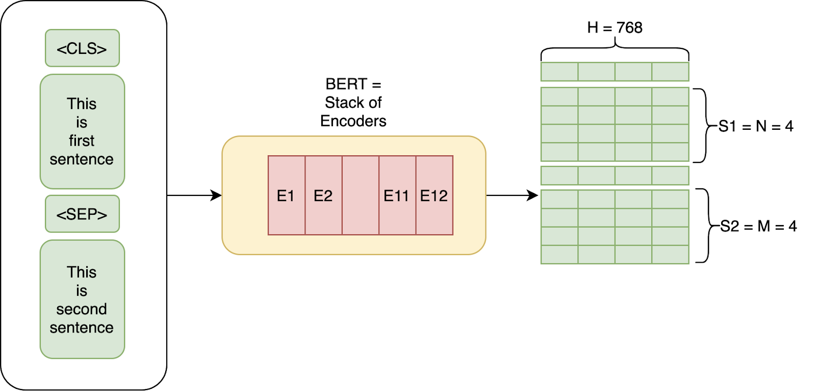
BERT is a Transformer-based model built on a stack of encoders designed to learn relationships between words in a sentence. Instead of processing text from left to right like older architectures, it reads entire sequences at once to form contextual understanding.
The original paper introduced two primary configurations:
While both versions deliver strong performance, BERT Large provides better language understanding at the cost of significantly higher computational and memory requirements. Fine-tuning BERT Large on large datasets can easily saturate a multi-GPU workstation or node with high VRAM capacity.
At its core, BERT converts every token (word or subword) into a 768-dimensional vector that represents meaning within its context. These embeddings can then be applied to multiple downstream tasks via finetuning:
Because BERT is pre-trained on massive text corpora, it can be fine-tuned for new workloads with less labeled data. However, fine-tuning still involves extensive retraining, making high-performance GPUs or multi-core CPUs valuable for reducing training time. View our Deep Learning Benchmark which feature BERT Base and BERT Large!
Training, inferencing, and fine-tuning Agentic AI, LLMs, and traditional AI models on massive datasets can be accelerated exponentially with the right system. We provide the tool to propel and accelerate your research.
Configure NowBERT is built on a Transformer encoder, a deep neural network architecture that uses self-attention to understand relationships between words. Instead of processing text sequentially like RNNs or LSTMs, BERT evaluates every token in parallel and captures dependencies across the entire sequence in parallel.
Each Transformer encoder layer includes three main operations:
These encoders are stacked repeatedly, forming BERT’s deep contextual network.
Since its release, researchers have developed optimized versions like DistilBERT, ALBERT, and RoBERTa, often referred to as Modern BERTs. These models retain the same Transformer structure but emphasize efficiency and training improvements:
For real-world workloads, choosing between BERT Base, Large, or modern variants depends on available compute and latency goals. Tasks that demand high accuracy, like document retrieval or conversational AI, benefit from larger architectures on GPU-accelerated servers, while edge or latency-sensitive deployments favor distilled models.
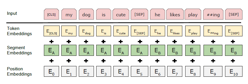
BERT doesn’t take raw text as input. Instead, it relies on a structured and tokenized format that allows it to handle multiple sentences and relationships between them.
The first step is WordPiece tokenization, which breaks text into sub-word units. This approach limits vocabulary size and helps handle rare or unseen words. For example, the word “playing” might be split into “play” and “##ing,” ensuring that BERT can understand variations of a root word like plays, played, or player.
BERT adds specific tokens to help the model interpret sentence structure:
For example, this sentence would become:
"My dog is cute. He likes playing."

A combination of three learned embeddings represents each token:
The final input vector for each token is the sum of these three embeddings. This composite input enables BERT to understand both the meaning and structure of text simultaneously.
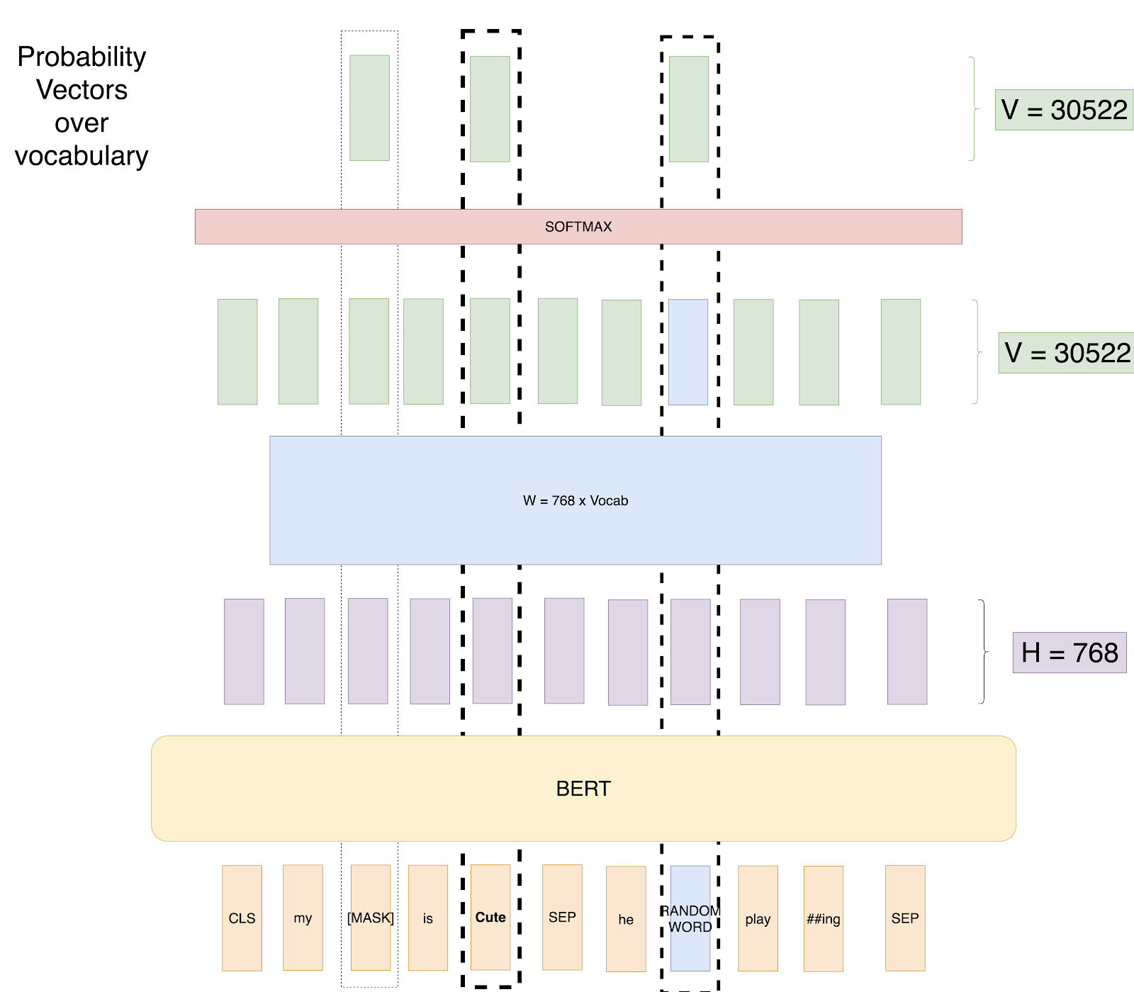
BERT’s training process is what makes it uniquely powerful. Instead of learning language patterns in one direction, it learns from both sides of a word simultaneously. This pre-training is performed on massive text corpora like Wikipedia and BooksCorpus, creating a deeply contextual understanding of language before fine-tuning for specific tasks.
BERT learns to predict missing words in a sentence. During training, about 15% of the tokens are selected for prediction using the following strategy:
This forces the model to infer meaning from the surrounding context instead of memorizing words. For example:
“My [MASK] is CUTE (unmasked). He [Random Word] playing.”
BERT learns to predict that the Masked Word is likely dog or cat, depending on context. This method enables bidirectional learning, allowing BERT to understand relationships between words in a way traditional left-to-right models could not.
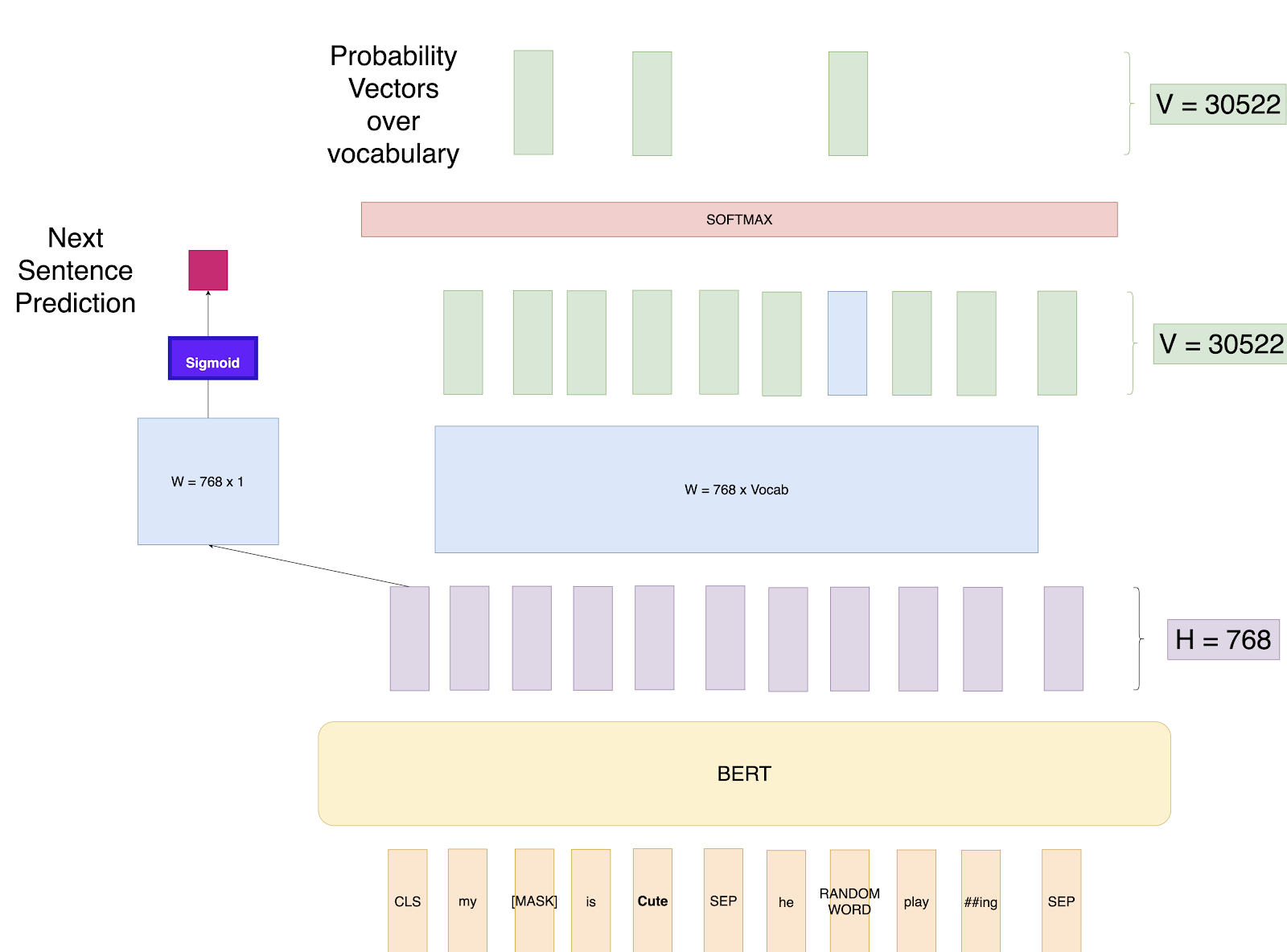
Alongside MLM, BERT also learns how sentences relate to each other. In this task, the model is fed two sentences:
The model predicts whether the second sentence is logically connected to the first. NSP improves BERT’s ability to handle tasks involving sentence relationships, such as question answering or reading comprehension.
Training BERT from scratch is extremely resource intensive. BERT Large, for instance, was trained on Google TPU with hundreds of cores running in parallel. Reproducing this at scale requires:
Running BERT Base on consumer GPUs is manageable, but BERT Large and Modern BERTs with long context windows can push memory usage past 20 GB. We would recommend the NVIDIA RTX PRO Blackwell series of GPUs.
Optimized inference often leverages tensor core GPUs or accelerators with mixed-precision support to maintain throughput without compromising accuracy. For organizations deploying large-scale NLP workloads, multi-GPU clusters or dedicated inference servers are essential for maintaining real-time performance.
Even fine-tuning on domain-specific datasets can take hours or days, depending on sequence length and model variant. For research institutions or enterprises, pre-trained checkpoints combined with scalable GPU servers are the most practical approach to harnessing BERT’s power.
With the latest CPUs and most powerful GPUs available, accelerate your deep learning and AI project optimized to your deployment, budget, and desired performance!
Configure NowOnce pre-trained, BERT can be adapted to specific workloads by adding lightweight task-specific layers and fine-tuning the entire model. This versatility makes it suitable for a wide range of enterprise NLP applications.
Fine-tuning often requires less data but still demands strong compute throughput:
Deploying BERT workloads at scale involves GPU servers or inference accelerators with optimized deep learning frameworks like TensorRT or ONNX Runtime.
Each task benefits from BERT’s deep contextual embeddings, which already encode syntactic and semantic information learned during pre-training.
BERT set a new standard for understanding natural language and continues to influence every major NLP architecture today. Its Transformer-based design enables deep contextual reasoning that outperforms older embedding models across nearly every language task.
Key points to remember:
For organizations deploying NLP systems, investing in high-performance GPU servers or clusters ensures BERT and its successors can deliver real-time insights with maximum efficiency. Whether for research, AI-driven customer support, or content intelligence, optimized infrastructure is key to unlocking the full potential of Transformer models.
BERT changed the way machines interpret human language. Short for Bidirectional Encoder Representations from Transformers, it allows models to understand context by reading text in both directions. While BERT is not the main focus of today’s LLMs, it is still a prevalent AI technology.
When BERT was introduced, it quickly became a benchmark model for Natural Language Processing (NLP) tasks. These workloads rely heavily on deep attention mechanisms that require high-throughput compute. Training or fine-tuning BERT efficiently often depends on GPU-accelerated servers capable of parallelizing massive matrix operations.
We will go over the BERT architectures, how it was trained, common applications, as well as offer hardware recommendations.
BERT is a Transformer-based model built on a stack of encoders designed to learn relationships between words in a sentence. Instead of processing text from left to right like older architectures, it reads entire sequences at once to form contextual understanding.
The original paper introduced two primary configurations:
While both versions deliver strong performance, BERT Large provides better language understanding at the cost of significantly higher computational and memory requirements. Fine-tuning BERT Large on large datasets can easily saturate a multi-GPU workstation or node with high VRAM capacity.
At its core, BERT converts every token (word or subword) into a 768-dimensional vector that represents meaning within its context. These embeddings can then be applied to multiple downstream tasks via finetuning:
Because BERT is pre-trained on massive text corpora, it can be fine-tuned for new workloads with less labeled data. However, fine-tuning still involves extensive retraining, making high-performance GPUs or multi-core CPUs valuable for reducing training time. View our Deep Learning Benchmark which feature BERT Base and BERT Large!
Training, inferencing, and fine-tuning Agentic AI, LLMs, and traditional AI models on massive datasets can be accelerated exponentially with the right system. We provide the tool to propel and accelerate your research.
Configure NowBERT is built on a Transformer encoder, a deep neural network architecture that uses self-attention to understand relationships between words. Instead of processing text sequentially like RNNs or LSTMs, BERT evaluates every token in parallel and captures dependencies across the entire sequence in parallel.
Each Transformer encoder layer includes three main operations:
These encoders are stacked repeatedly, forming BERT’s deep contextual network.
Since its release, researchers have developed optimized versions like DistilBERT, ALBERT, and RoBERTa, often referred to as Modern BERTs. These models retain the same Transformer structure but emphasize efficiency and training improvements:
For real-world workloads, choosing between BERT Base, Large, or modern variants depends on available compute and latency goals. Tasks that demand high accuracy, like document retrieval or conversational AI, benefit from larger architectures on GPU-accelerated servers, while edge or latency-sensitive deployments favor distilled models.
BERT doesn’t take raw text as input. Instead, it relies on a structured and tokenized format that allows it to handle multiple sentences and relationships between them.
The first step is WordPiece tokenization, which breaks text into sub-word units. This approach limits vocabulary size and helps handle rare or unseen words. For example, the word “playing” might be split into “play” and “##ing,” ensuring that BERT can understand variations of a root word like plays, played, or player.
BERT adds specific tokens to help the model interpret sentence structure:
For example, this sentence would become:
"My dog is cute. He likes playing."
A combination of three learned embeddings represents each token:
The final input vector for each token is the sum of these three embeddings. This composite input enables BERT to understand both the meaning and structure of text simultaneously.
BERT’s training process is what makes it uniquely powerful. Instead of learning language patterns in one direction, it learns from both sides of a word simultaneously. This pre-training is performed on massive text corpora like Wikipedia and BooksCorpus, creating a deeply contextual understanding of language before fine-tuning for specific tasks.
BERT learns to predict missing words in a sentence. During training, about 15% of the tokens are selected for prediction using the following strategy:
This forces the model to infer meaning from the surrounding context instead of memorizing words. For example:
“My [MASK] is CUTE (unmasked). He [Random Word] playing.”
BERT learns to predict that the Masked Word is likely dog or cat, depending on context. This method enables bidirectional learning, allowing BERT to understand relationships between words in a way traditional left-to-right models could not.
Alongside MLM, BERT also learns how sentences relate to each other. In this task, the model is fed two sentences:
The model predicts whether the second sentence is logically connected to the first. NSP improves BERT’s ability to handle tasks involving sentence relationships, such as question answering or reading comprehension.
Training BERT from scratch is extremely resource intensive. BERT Large, for instance, was trained on Google TPU with hundreds of cores running in parallel. Reproducing this at scale requires:
Running BERT Base on consumer GPUs is manageable, but BERT Large and Modern BERTs with long context windows can push memory usage past 20 GB. We would recommend the NVIDIA RTX PRO Blackwell series of GPUs.
Optimized inference often leverages tensor core GPUs or accelerators with mixed-precision support to maintain throughput without compromising accuracy. For organizations deploying large-scale NLP workloads, multi-GPU clusters or dedicated inference servers are essential for maintaining real-time performance.
Even fine-tuning on domain-specific datasets can take hours or days, depending on sequence length and model variant. For research institutions or enterprises, pre-trained checkpoints combined with scalable GPU servers are the most practical approach to harnessing BERT’s power.
With the latest CPUs and most powerful GPUs available, accelerate your deep learning and AI project optimized to your deployment, budget, and desired performance!
Configure NowOnce pre-trained, BERT can be adapted to specific workloads by adding lightweight task-specific layers and fine-tuning the entire model. This versatility makes it suitable for a wide range of enterprise NLP applications.
Fine-tuning often requires less data but still demands strong compute throughput:
Deploying BERT workloads at scale involves GPU servers or inference accelerators with optimized deep learning frameworks like TensorRT or ONNX Runtime.
Each task benefits from BERT’s deep contextual embeddings, which already encode syntactic and semantic information learned during pre-training.
BERT set a new standard for understanding natural language and continues to influence every major NLP architecture today. Its Transformer-based design enables deep contextual reasoning that outperforms older embedding models across nearly every language task.
Key points to remember:
For organizations deploying NLP systems, investing in high-performance GPU servers or clusters ensures BERT and its successors can deliver real-time insights with maximum efficiency. Whether for research, AI-driven customer support, or content intelligence, optimized infrastructure is key to unlocking the full potential of Transformer models.
