Artificial Intelligence
GNN Demo Using PyTorch Lightning and PyTorch Geometric
March 15, 2022
20 min read

In the world of deep learning, Python rules. But while the Python programming language on its own is very fast to develop in, a so-called “high-productivity” language, execution speed pales in comparison to compiled and lower-level languages like C++ or FORTRAN.
One of the fundamental drivers of the neural network renaissance of the 2010s to today, aka the advent of deep learning, is scaling up model and dataset sizes to take advantage of fast hardware.
The almighty general-purpose graphics processing unit, or just plain GPU for short, is the most well-known hardware accelerator and is well-suited to the massively parallel-izable mathematical primitives that neural networks are built out of, but there are many other more specialized accelerators out there as well.
Specialized deep learning hardware is no longer the sole purview of prototypes and startup pitches either; from TPUs to IPUs, there are plenty of specialized chips that are commercially available for running deep learning models, usually in a cloud offering.
To take advantage of the latest in deep learning hardware, you need to develop models that can be ported to a library that supports the hardware. This is a significant advantage of PyTorch Lightning.
In typical use, PyTorch Lightning not only makes it relatively simple to scale models to run on exotic hardware like TPUs, but also simplifies the process of switching between run-of-the-mill CPU and GPU and makes distributed training much easier as well.
It’s often been said that the most scarce resource in developing a deep learning project is the time and attention of human developers, rather than computer time. PyTorch Lightning is an additional layer of tools and abstractions to simplify the aspects of deep learning that require manual developer attention, on top of all the familiar productivity-enhancing features of PyTorch and Python.
As you’re likely to come across in the Lightning documentation and blog, a point of pride for Lightning developers is that the library doesn’t reduce the control you have over models, training, or deployment.
In this article, we focus on the productivity enhancing features of Lightning by developing models and training for an example project of graph classification with a graph convolution network. We'll try to get a feel for the potential productivity, interpretability, and reproducibility advantages of Lightning.
Although we focus on reducing boilerplate and simplifying training with the LightningModule class, Lightning offers a number of more advanced capabilities like scheduling and optimizing learning rates, using specialized loggers, or streamlining dstributed training strategies. By the end, I hope that you’ll be equipped to make a well-informed decision about whether Lightning is a good fit for your next project, or at least you’ll know where to look and what questions to ask.
To make things more exciting, we won’t compare just PyTorch to just PyTorch Lightning. Instead, we’ll take a look at a slightly more interesting and specialized use case: graph classification with graph convolutional networks.
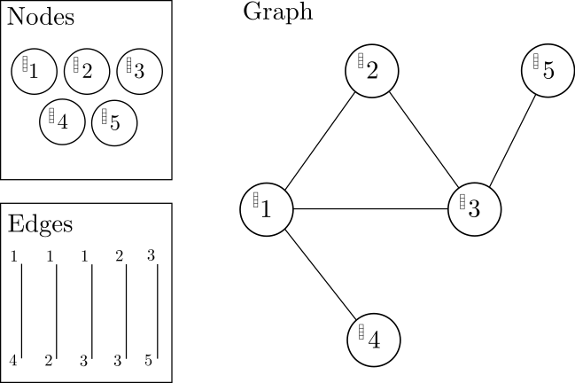
Image CC-BY 4.0 Irhum Shafkat at irhum.pubpub.org
We’ll use the popular graph deep learning framework PyTorch Geometric to build our model, and we'll also use a built-in dataset call "PROTEINS" in TUDataset.
This dataset includes cleaned versions of the datasets as described in a paper by Ivanov et al. in 2019, and it’s available as part of PyTorch Geometric’s datasets module. Alternatively you can classify a graph version of MNIST, or replace the dataset used in the code below with your graph classification problem of choice.
As a graph deep learning library, PyTorch Geometric has to bundle multiple graphs into a single set of matrices representing edges (the adjacency matrix), node characteristics, edge attributes (if applicable), and graph indices. This means that instead of passing a simple tensor representing input images or vectors, batches for graph deep learning with this library are a little more complicated, and are represented as a named tuple.
Will this atypical data structure throw a wrench in the smooth development experience of working with Lightning?
Interested in a system to run graph neural networks on?
Learn more about Exxact AI workstations starting around $5,500
We'll use the popular graph deep learning library PyTorch Geometric in tandem with Lightning, and we'll keep this demo project contained in its own virtual environment.
The instructions are intended for the virtualenv, but you should have no problems adapting them to work with Anaconda or your favorite virtual environment manager.
virtualenv ptl_vs_pl --python=python3
source ptl_vs_pl/bin/activate

# install pytorch lightning
pip install pytorch-lightning

# install pytorch geometric (CUDA 10.2, pytorch 1.10)
pip install torch-scatter -f https://data.pyg.org/whl/torch-1.10.0+cu102.html
Pip install torch-sparse -f https://data.pyg.org/whl/torch-1.10.0+cu102.html
pip install torch-cluster -f https://data.pyg.org/whl/torch-1.10.0+cu102.html
pip install  torch-spline-conv -f https://data.pyg.org/whl/torch-1.10.0+cu102.html
pip install torch-geometric -f https://data.pyg.org/whl/torch-1.10.0+cu102.html

# for cuda 11.3 use -f https://data.pyg.org/whl/torch-1.10.0+cu113.html
# for cpu only use -f https://data.pyg.org/whl/torch-1.10.0+cpu.html
Next we'll begin building our project. This simple demo will consist of imports, model definition, training loop definition, and a section for instantiating the dataset and dataloader and calling the training loop.
The first thing we need to do when writing our modules for graph classification is imports.
This section is shared between both the Lightning and standard PyTorch+Geometric versions of our project, except for the lines with comments specifying otherwise in the lines below.
import time
import numpy as np
import torch
from torch.nn import Dropout, Linear, ReLU
import torch_geometric
from torch_geometric.datasets import TUDataset, GNNBenchmarkDataset
from torch_geometric.loader import DataLoader
from torch_geometric.nn import GCNConv, Sequential, global_mean_pool

# this import is only used in the plain PyTorch+Geometric version
from torch.utils.tensorboard import SummaryWriter

# these imports are only used in the Lighning version
import pytorch_lightning as pl
import torch.nn.functional as F
We'll start by building a graph convolutional network in PyTorch+Geometric. Our PlainGCN model inherits from the stand nn.Module class in torch, and uses the Sequential model class from PyTorch Geometric to define the forward pass.
The Sequential class from torch_geometric.nn differs somewhat from the standard version in torch.nn, but aside from that this model will look very similar to any other torch model inheriting from nn.Module.
Geometric's Sequential models take additional string arguments to define what the various modules making up the model will do with the inputs. This feels a lot like the typical process of overriding the forward function in standard PyTorch models.
Indeed, defining the model’s forward pass in the Sequential model means all we have to do when we actually get to forward is parse the batch data (including edges, node features, and batch indices) and pass these to the Sequential model.
class PlainGCN(torch.nn.Module):

    def __init__(self, **kwargs):
        super(PlainGCN, self).__init__()


        self.num_features = kwargs["num_features"] \
            if "num_features" in kwargs.keys() else 3

        self.num_classes = kwargs["num_classes"] \
            if "num_classes" in kwargs.keys() else 2


        # hidden layer node features
        self.hidden = 256

        self.model = Sequential("x, edge_index, batch_index", [\
                (GCNConv(self.num_features, self.hidden), \
                    "x, edge_index -> x1"),
                (ReLU(), "x1 -> x1a"),\
                (Dropout(p=0.5), "x1a -> x1d"),\
                (GCNConv(self.hidden, self.hidden), "x1d, edge_index -> x2"), \
                (ReLU(), "x2 -> x2a"),\
                (Dropout(p=0.5), "x2a -> x2d"),\
                (GCNConv(self.hidden, self.hidden), "x2d, edge_index -> x3"), \
                (ReLU(), "x3 -> x3a"),\
                (Dropout(p=0.5), "x3a -> x3d"),\
                (GCNConv(self.hidden, self.hidden), "x3d, edge_index -> x4"), \
                (ReLU(), "x4 -> x4a"),\
                (Dropout(p=0.5), "x4a -> x4d"),\
                (GCNConv(self.hidden, self.hidden), "x4d, edge_index -> x5"), \
                (ReLU(), "x5 -> x5a"),\
                (Dropout(p=0.5), "x5a -> x5d"),\
                (global_mean_pool, "x5d, batch_index -> x6"),\
                (Linear(self.hidden, self.num_classes), "x6 -> x_out")])

    def forward(self, graph_data):


        x, edge_index, batch = graph_data.x, graph_data.edge_index,\
                    graph_data.batch

        x_out = self.model(x, edge_index, batch)

        return x_out
Building the model for Lightning is a little more involved, but there's a good reason for that. In PyTorch Lightning, training is centered on the LightningModule class and training, validation, and logging are all part of the model itself.
The first thing to notice is that the model inherits from the LightningModule instead of the standard nn.Module from PyTorch.
After that, the model is defined in the same way as the PyTorch+Geometric only version, until we get to the Lightning-specific training_step, validation_step, and validation_epoch_end.
Those three functions define what the model does during training, and this LightningModule-centered approach to training can significantly decrease the amount of boilerplate involved.
class LightningGCN(pl.LightningModule):

    def __init__(self, **kwargs):
        super(LightningGCN, self).__init__()

        self.num_features = kwargs["num_features"] \
                    if "num_features" in kwargs.keys() else 3
        self.num_classes = kwargs["num_classes"] \
                    if "num_classes" in kwargs.keys() else 2

        # hidden layer node features
        self.hidden = 256

        self.model = Sequential("x, edge_index, batch_index", [\
                (GCNConv(self.num_features, self.hidden), \
                    "x, edge_index -> x1"),
                (ReLU(), "x1 -> x1a"),\
                (Dropout(p=0.5), "x1a -> x1d"),\
                (GCNConv(self.hidden, self.hidden), "x1d, edge_index -> x2"), \
                (ReLU(), "x2 -> x2a"),\
                (Dropout(p=0.5), "x2a -> x2d"),\
                (GCNConv(self.hidden, self.hidden), "x2d, edge_index -> x3"), \
                (ReLU(), "x3 -> x3a"),\
                (Dropout(p=0.5), "x3a -> x3d"),\
                (GCNConv(self.hidden, self.hidden), "x3d, edge_index -> x4"), \
                (ReLU(), "x4 -> x4a"),\
                (Dropout(p=0.5), "x4a -> x4d"),\
                (GCNConv(self.hidden, self.hidden), "x4d, edge_index -> x5"), \
                (ReLU(), "x5 -> x5a"),\
                (Dropout(p=0.5), "x5a -> x5d"),\
                (global_mean_pool, "x5d, batch_index -> x6"),\
                (Linear(self.hidden, self.num_classes), "x6 -> x_out")])


    def forward(self, x, edge_index, batch_index):

        x_out = self.model(x, edge_index, batch_index)

        return x_out

    def training_step(self, batch, batch_index):

        x, edge_index = batch.x, batch.edge_index
        batch_index = batch.batch

        x_out = self.forward(x, edge_index, batch_index)

        loss = F.cross_entropy(x_out, batch.y)

        # metrics here
        pred = x_out.argmax(-1)
        label = batch.y
        accuracy = (pred == label).sum() / pred.shape[0]

        self.log("loss/train", loss)
        self.log("accuracy/train", accuracy)

        return loss

    def validation_step(self, batch, batch_index):
        x, edge_index = batch.x, batch.edge_index
        batch_index = batch.batch

        x_out = self.forward(x, edge_index, batch_index)

        loss = F.cross_entropy(x_out, batch.y)

        pred = x_out.argmax(-1)

        return x_out, pred, batch.y

    def validation_epoch_end(self, validation_step_outputs):

        val_loss = 0.0
        num_correct = 0
        num_total = 0

        for output, pred, labels in validation_step_outputs:

            val_loss += F.cross_entropy(output, labels, reduction="sum")

            num_correct += (pred == labels).sum()
            num_total += pred.shape[0]


            val_accuracy = num_correct / num_total
            val_loss = val_loss / num_total

        self.log("accuracy/val", val_accuracy)
        self.log("loss/val", val_loss)

    def configure_optimizers(self):
        return torch.optim.Adam(self.parameters(), lr = 3e-4)
For our standard PyTorch+Geometric development scenario, we’ll define evaluation functions and logging manually. Of course, you may usually use another helper library like tensorboard to log progress and checkpoints, but we’re comparing training with Lightning to PyTorch alone for this demo.
People sometimes call the tendency to roll-your-own and implement standard logging and other functionality manually for every project by coding it yourself as “being a hero” also known as "being a masochist."
This tends to lead to a code-base with lots of boilerplate, and as they say you either burn out as a hero or live long enough to - not want to be a hero anymore, due to the abject boredom of making minute changes to standard boilerplate for each new piece of a project.
Here's the roll-your-own evaluation function using plain PyTorch, with a little TensorBoard for building a dashboard for progress logs:
def evaluate(model, test_loader, save_results=True, tag="_default", verbose=False):

    # get test accuracy score

    num_correct = 0.
    num_total = 0.

    my_device = "cuda" if torch.cuda.is_available() else "cpu"
    criterion = torch.nn.CrossEntropyLoss(reduction="sum")

    model.eval()
    total_loss = 0
    total_batches = 0

    for batch in test_loader:

        pred = model(batch.to(my_device))

        loss = criterion(pred, batch.y.to(my_device))

        num_correct += (pred.argmax(dim=1) == batch.y).sum()
        num_total += pred.shape[0]

        total_loss += loss.detach()
        total_batches += batch.batch.max()

    test_loss = total_loss / total_batches
    test_accuracy = num_correct / num_total

    if verbose:
        print(f"accuracy = {test_accuracy:.4f}")

    results = {"accuracy": test_accuracy, \
        "loss": test_loss, \
        "tag": tag }

    return results
The first thing you'll notice about the evaluation function for the Lightning version is that it is significantly shorter than the one above. Here it is:
Oh wait, we don’t need a separate evaluation function. That functionality is already included in our validation_step and validation_epoch_end functions of the LightningModule class.
Now let’s define the training loop. We’ll wrap this up as a function and make evaluation calls and save progress from within one big loop through the batches of the training dataloader.
def train_model(model, train_loader, criterion, optimizer, num_epochs=1000, \
        verbose=True, val_loader=None, save_tag="default_run_"):

    ## call validation function and print progress at each epoch end
    display_every = 1 #num_epochs // 10
    my_device = "cuda" if torch.cuda.is_available() else "cpu"
    model.to(my_device)

    # we'll log progress to tensorboard
    log_dir = f"lightning_logs/plain_model_{str(int(time.time()))[-8:]}/"
    writer = SummaryWriter(log_dir=log_dir)

    t0 = time.time()
    for epoch in range(num_epochs):

        total_loss = 0.0
        batch_count = 0
        for batch in train_loader:
        optimizer.zero_grad()

        pred = model(batch.to(my_device))
        loss = criterion(pred, batch.y.to(my_device))
        loss.backward()

        optimizer.step()

        total_loss += loss.detach()
        batch_count += 1

    mean_loss = total_loss / batch_count

    writer.add_scalar("loss/train", mean_loss, epoch)

    if epoch % display_every == 0:
        train_results = evaluate(model, train_loader, \
        tag=f"train_ckpt_{epoch}_", verbose=False)
        train_loss = train_results["loss"]
        train_accuracy = train_results["accuracy"]

    if verbose:
        print(f"training loss & accuracy at epoch {epoch} = "\
        f"{train_loss:.4f} & {train_accuracy:.4f}")

    if val_loader is not None:
        val_results = evaluate(model, val_loader, \
        tag=f"val_ckpt_{epoch}_", verbose=False)
        val_loss = val_results["loss"]
        val_accuracy = val_results["accuracy"]

    if verbose:
        print(f"val. loss & accuracy at epoch {epoch} = "\
        f"{val_loss:.4f} & {val_accuracy:.4f}")
        else:
        val_loss = float("Inf")
        val_acc = - float("Inf")

    writer.add_scalar("loss/train_eval", train_loss, epoch)
    writer.add_scalar("loss/val", val_loss, epoch)
    writer.add_scalar("accuracy/train", train_accuracy, epoch)
    writer.add_scalar("accuracy/val", val_accuracy, epoch)
As earlier with our evaluation function, we’ve already defined the Lightning equivalent as part of the LightningModule model.
In this section, we have the code for instantiating a built-in dataset from PyTorch Geometric, which will take a few minutes to download the first time you run it.
This section also shuffles and splits the dataset and instantiates the dataloaders we’ll need for training and validation, and finally calls the training function (for standard PyTorch) or instantiates a Trainer object and calls fit in the Lightning version.
The first part, where the dataset is downloaded, shuffled, and split, is the same for each version.
You can choose whether you'd like to train on the TUDataset PROTEINs dataset or on a graph version of MNIST from GNNBenchmarkDataset, the latter of which has more samples and will take a little longer to train. You can also substitute your graph classification problem of choice if you prefer.
if __name__ == "__main__":

    # choose the TUDataset or MNIST,
    # or another graph classification problem if preferred
    dataset = TUDataset(root="./tmp", name="PROTEINS")
    #dataset = GNNBenchmarkDataset(root="./tmp", name="MNIST")

    # shuffle dataset and get train/validation/test splits
    dataset = dataset.shuffle()

    num_samples = len(dataset)
    batch_size = 32

    num_val = num_samples // 10

    val_dataset = dataset[:num_val]
    test_dataset = dataset[num_val:2 * num_val]
    train_dataset = dataset[2 * num_val:]

    train_loader = DataLoader(train_dataset, batch_size=batch_size)
    test_loader = DataLoader(test_dataset, batch_size=batch_size)
    val_loader = DataLoader(val_dataset, batch_size=batch_size)

    for batch in train_loader:
    break

    num_features = batch.x.shape[1]
    num_classes = dataset.num_classes
At this point we're ready to instantiate our model and call a training function, and this is where the Lightning and the standard PyTorch versions diverge. We'll go over the standard version first.
    plain_model = PlainGCN(num_features=num_features, num_classes=num_classes)
    lr = 1e-5
    num_epochs = 2500

    criterion = torch.nn.CrossEntropyLoss(reduction="sum")
    optimizer = torch.optim.Adam(plain_model.parameters(), lr=lr)

    train_model(plain_model, train_loader, criterion, optimizer,\
            num_epochs=num_epochs, verbose=True, \
            val_loader=val_loader)
In the Lightning version, we use the Trainer class to call fit and orchestrate training. This will handle calls to all the training and validation functionality we built into the LightningModule model.
Notice the argument gpus=[0] we use when instantiating the Trainer object, this is the only thing we need to incorporate to make sure the model and all data tensors end up on the GPU for training.
    lightning_model = LightningGCN(num_features=num_features, \
            num_classes=num_classes)

    num_epochs = 2500
    val_check_interval = len(train_loader)

    trainer = pl.Trainer(max_epochs = num_epochs, \
            val_check_interval=val_check_interval, gpus=[0])
    trainer.fit(lightning_model, train_loader, val_loader)
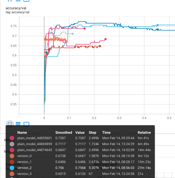
Both versions of our graph convolutional model log to tensorboard, so we can easily compare experimental runs. Over a few different runs, our validation accuracy tops out at just over 75%, which is in the ballpark of what was reported for GCNs in the publication by Ivanov et al.
It was surprising how easy it was to integrate the atypical data structure of graph batches (a named tuple) used by PyTorch Geometric into a model based on the LightningModule from PyTorch Lightning.
This is a strong point of Lightning: although you can take advantage of a number of built-in abstractions and features to make development more productive, Lightning retains the flexibility to tackle relatively specialized problems like deep learning on graphs.
We also encountered a few interesting and helpful surprises while working on this demonstration project.
In PyTorch Lightning, the Trainer object handles allocation to different hardware accelerators like GPUs, TPUs, and IPUs. This makes it exceptionally easy to train on a local GPU with the addition of a single argument to instantiating the trainer, and it's also a lot easier to scale up to ASIC hardware accelerators like Google's TPUs or Graphcore's IPUs.
In standard PyTorch, moving data tensors onto the hardware you want to use is more manual, which can be a source of frustration for models with multiple hierarchical modules or strange architectures.
We are well aware of the need to move tensors where they need to be, but we still encountered a runtime error when we forgot to bring a tensor from the validation dataloader onto the GPU in an evaluation call.
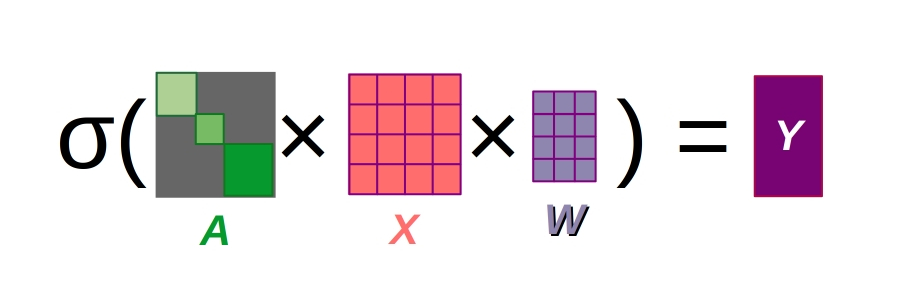
Public domain image of graph convolutions with several graphs combined into a single adjacency matrix
Another convenience working with Lightning was a warning about using too few workers in the dataloader.
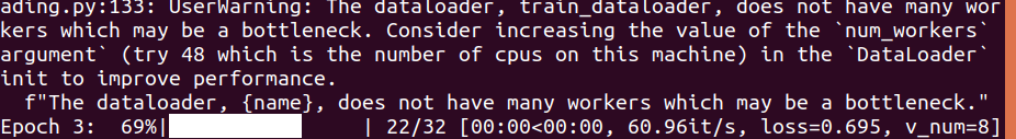
Deep learning on graphs can have a substantial pre-processing overhead, especially when dataset samples are shuffled for each epoch.
This is because the individual graphs are typically arranged into a single set of matrices defining graph connections and features, as in the image above. Helpfully, Lightning warned us about this and we increased the workers to a more reasonable 20.
So, is it worth learning yet another deep learning library to enhance your projects? In the case of PyTorch Lightning, the answer is yes.
Lightning is just PyTorch+, you don’t have to learn a large set of new APIs to start taking advantage of the extra convenience and features of Lightning. It retains the flexibility of pure PyTorch, so you can still approach complex and relatively specialized problems.
Lightning is a great way to reduce the amount of boilerplate code for each new project and make hardware acceleration (even on different devices) easy.
Lightning also plays nice with other libraries, as we experienced first hand by integrating graph convolution layers and graph dataloaders from PyTorch Geometric in a LightningModule model. This flexibility is the result of a focus on research.
Whereas most other libraries aimed at simplifying and enhancing PyTorch focus on the use case of working on known problems (i.e. they are more focused on a data science use case), Lightning is built for scientists and engineers that need to build something new.
Have any questions?
Contact Exxact Today
In the world of deep learning, Python rules. But while the Python programming language on its own is very fast to develop in, a so-called “high-productivity” language, execution speed pales in comparison to compiled and lower-level languages like C++ or FORTRAN.
One of the fundamental drivers of the neural network renaissance of the 2010s to today, aka the advent of deep learning, is scaling up model and dataset sizes to take advantage of fast hardware.
The almighty general-purpose graphics processing unit, or just plain GPU for short, is the most well-known hardware accelerator and is well-suited to the massively parallel-izable mathematical primitives that neural networks are built out of, but there are many other more specialized accelerators out there as well.
Specialized deep learning hardware is no longer the sole purview of prototypes and startup pitches either; from TPUs to IPUs, there are plenty of specialized chips that are commercially available for running deep learning models, usually in a cloud offering.
To take advantage of the latest in deep learning hardware, you need to develop models that can be ported to a library that supports the hardware. This is a significant advantage of PyTorch Lightning.
In typical use, PyTorch Lightning not only makes it relatively simple to scale models to run on exotic hardware like TPUs, but also simplifies the process of switching between run-of-the-mill CPU and GPU and makes distributed training much easier as well.
It’s often been said that the most scarce resource in developing a deep learning project is the time and attention of human developers, rather than computer time. PyTorch Lightning is an additional layer of tools and abstractions to simplify the aspects of deep learning that require manual developer attention, on top of all the familiar productivity-enhancing features of PyTorch and Python.
As you’re likely to come across in the Lightning documentation and blog, a point of pride for Lightning developers is that the library doesn’t reduce the control you have over models, training, or deployment.
In this article, we focus on the productivity enhancing features of Lightning by developing models and training for an example project of graph classification with a graph convolution network. We'll try to get a feel for the potential productivity, interpretability, and reproducibility advantages of Lightning.
Although we focus on reducing boilerplate and simplifying training with the LightningModule class, Lightning offers a number of more advanced capabilities like scheduling and optimizing learning rates, using specialized loggers, or streamlining dstributed training strategies. By the end, I hope that you’ll be equipped to make a well-informed decision about whether Lightning is a good fit for your next project, or at least you’ll know where to look and what questions to ask.
To make things more exciting, we won’t compare just PyTorch to just PyTorch Lightning. Instead, we’ll take a look at a slightly more interesting and specialized use case: graph classification with graph convolutional networks.
Image CC-BY 4.0 Irhum Shafkat at irhum.pubpub.org
We’ll use the popular graph deep learning framework PyTorch Geometric to build our model, and we'll also use a built-in dataset call "PROTEINS" in TUDataset.
This dataset includes cleaned versions of the datasets as described in a paper by Ivanov et al. in 2019, and it’s available as part of PyTorch Geometric’s datasets module. Alternatively you can classify a graph version of MNIST, or replace the dataset used in the code below with your graph classification problem of choice.
As a graph deep learning library, PyTorch Geometric has to bundle multiple graphs into a single set of matrices representing edges (the adjacency matrix), node characteristics, edge attributes (if applicable), and graph indices. This means that instead of passing a simple tensor representing input images or vectors, batches for graph deep learning with this library are a little more complicated, and are represented as a named tuple.
Will this atypical data structure throw a wrench in the smooth development experience of working with Lightning?
Interested in a system to run graph neural networks on?
Learn more about Exxact AI workstations starting around $5,500
We'll use the popular graph deep learning library PyTorch Geometric in tandem with Lightning, and we'll keep this demo project contained in its own virtual environment.
The instructions are intended for the virtualenv, but you should have no problems adapting them to work with Anaconda or your favorite virtual environment manager.
virtualenv ptl_vs_pl --python=python3
source ptl_vs_pl/bin/activate

# install pytorch lightning
pip install pytorch-lightning

# install pytorch geometric (CUDA 10.2, pytorch 1.10)
pip install torch-scatter -f https://data.pyg.org/whl/torch-1.10.0+cu102.html
Pip install torch-sparse -f https://data.pyg.org/whl/torch-1.10.0+cu102.html
pip install torch-cluster -f https://data.pyg.org/whl/torch-1.10.0+cu102.html
pip install  torch-spline-conv -f https://data.pyg.org/whl/torch-1.10.0+cu102.html
pip install torch-geometric -f https://data.pyg.org/whl/torch-1.10.0+cu102.html

# for cuda 11.3 use -f https://data.pyg.org/whl/torch-1.10.0+cu113.html
# for cpu only use -f https://data.pyg.org/whl/torch-1.10.0+cpu.html
Next we'll begin building our project. This simple demo will consist of imports, model definition, training loop definition, and a section for instantiating the dataset and dataloader and calling the training loop.
The first thing we need to do when writing our modules for graph classification is imports.
This section is shared between both the Lightning and standard PyTorch+Geometric versions of our project, except for the lines with comments specifying otherwise in the lines below.
import time
import numpy as np
import torch
from torch.nn import Dropout, Linear, ReLU
import torch_geometric
from torch_geometric.datasets import TUDataset, GNNBenchmarkDataset
from torch_geometric.loader import DataLoader
from torch_geometric.nn import GCNConv, Sequential, global_mean_pool

# this import is only used in the plain PyTorch+Geometric version
from torch.utils.tensorboard import SummaryWriter

# these imports are only used in the Lighning version
import pytorch_lightning as pl
import torch.nn.functional as F
We'll start by building a graph convolutional network in PyTorch+Geometric. Our PlainGCN model inherits from the stand nn.Module class in torch, and uses the Sequential model class from PyTorch Geometric to define the forward pass.
The Sequential class from torch_geometric.nn differs somewhat from the standard version in torch.nn, but aside from that this model will look very similar to any other torch model inheriting from nn.Module.
Geometric's Sequential models take additional string arguments to define what the various modules making up the model will do with the inputs. This feels a lot like the typical process of overriding the forward function in standard PyTorch models.
Indeed, defining the model’s forward pass in the Sequential model means all we have to do when we actually get to forward is parse the batch data (including edges, node features, and batch indices) and pass these to the Sequential model.
class PlainGCN(torch.nn.Module):

    def __init__(self, **kwargs):
        super(PlainGCN, self).__init__()


        self.num_features = kwargs["num_features"] \
            if "num_features" in kwargs.keys() else 3

        self.num_classes = kwargs["num_classes"] \
            if "num_classes" in kwargs.keys() else 2


        # hidden layer node features
        self.hidden = 256

        self.model = Sequential("x, edge_index, batch_index", [\
                (GCNConv(self.num_features, self.hidden), \
                    "x, edge_index -> x1"),
                (ReLU(), "x1 -> x1a"),\
                (Dropout(p=0.5), "x1a -> x1d"),\
                (GCNConv(self.hidden, self.hidden), "x1d, edge_index -> x2"), \
                (ReLU(), "x2 -> x2a"),\
                (Dropout(p=0.5), "x2a -> x2d"),\
                (GCNConv(self.hidden, self.hidden), "x2d, edge_index -> x3"), \
                (ReLU(), "x3 -> x3a"),\
                (Dropout(p=0.5), "x3a -> x3d"),\
                (GCNConv(self.hidden, self.hidden), "x3d, edge_index -> x4"), \
                (ReLU(), "x4 -> x4a"),\
                (Dropout(p=0.5), "x4a -> x4d"),\
                (GCNConv(self.hidden, self.hidden), "x4d, edge_index -> x5"), \
                (ReLU(), "x5 -> x5a"),\
                (Dropout(p=0.5), "x5a -> x5d"),\
                (global_mean_pool, "x5d, batch_index -> x6"),\
                (Linear(self.hidden, self.num_classes), "x6 -> x_out")])

    def forward(self, graph_data):


        x, edge_index, batch = graph_data.x, graph_data.edge_index,\
                    graph_data.batch

        x_out = self.model(x, edge_index, batch)

        return x_out
Building the model for Lightning is a little more involved, but there's a good reason for that. In PyTorch Lightning, training is centered on the LightningModule class and training, validation, and logging are all part of the model itself.
The first thing to notice is that the model inherits from the LightningModule instead of the standard nn.Module from PyTorch.
After that, the model is defined in the same way as the PyTorch+Geometric only version, until we get to the Lightning-specific training_step, validation_step, and validation_epoch_end.
Those three functions define what the model does during training, and this LightningModule-centered approach to training can significantly decrease the amount of boilerplate involved.
class LightningGCN(pl.LightningModule):

    def __init__(self, **kwargs):
        super(LightningGCN, self).__init__()

        self.num_features = kwargs["num_features"] \
                    if "num_features" in kwargs.keys() else 3
        self.num_classes = kwargs["num_classes"] \
                    if "num_classes" in kwargs.keys() else 2

        # hidden layer node features
        self.hidden = 256

        self.model = Sequential("x, edge_index, batch_index", [\
                (GCNConv(self.num_features, self.hidden), \
                    "x, edge_index -> x1"),
                (ReLU(), "x1 -> x1a"),\
                (Dropout(p=0.5), "x1a -> x1d"),\
                (GCNConv(self.hidden, self.hidden), "x1d, edge_index -> x2"), \
                (ReLU(), "x2 -> x2a"),\
                (Dropout(p=0.5), "x2a -> x2d"),\
                (GCNConv(self.hidden, self.hidden), "x2d, edge_index -> x3"), \
                (ReLU(), "x3 -> x3a"),\
                (Dropout(p=0.5), "x3a -> x3d"),\
                (GCNConv(self.hidden, self.hidden), "x3d, edge_index -> x4"), \
                (ReLU(), "x4 -> x4a"),\
                (Dropout(p=0.5), "x4a -> x4d"),\
                (GCNConv(self.hidden, self.hidden), "x4d, edge_index -> x5"), \
                (ReLU(), "x5 -> x5a"),\
                (Dropout(p=0.5), "x5a -> x5d"),\
                (global_mean_pool, "x5d, batch_index -> x6"),\
                (Linear(self.hidden, self.num_classes), "x6 -> x_out")])


    def forward(self, x, edge_index, batch_index):

        x_out = self.model(x, edge_index, batch_index)

        return x_out

    def training_step(self, batch, batch_index):

        x, edge_index = batch.x, batch.edge_index
        batch_index = batch.batch

        x_out = self.forward(x, edge_index, batch_index)

        loss = F.cross_entropy(x_out, batch.y)

        # metrics here
        pred = x_out.argmax(-1)
        label = batch.y
        accuracy = (pred == label).sum() / pred.shape[0]

        self.log("loss/train", loss)
        self.log("accuracy/train", accuracy)

        return loss

    def validation_step(self, batch, batch_index):
        x, edge_index = batch.x, batch.edge_index
        batch_index = batch.batch

        x_out = self.forward(x, edge_index, batch_index)

        loss = F.cross_entropy(x_out, batch.y)

        pred = x_out.argmax(-1)

        return x_out, pred, batch.y

    def validation_epoch_end(self, validation_step_outputs):

        val_loss = 0.0
        num_correct = 0
        num_total = 0

        for output, pred, labels in validation_step_outputs:

            val_loss += F.cross_entropy(output, labels, reduction="sum")

            num_correct += (pred == labels).sum()
            num_total += pred.shape[0]


            val_accuracy = num_correct / num_total
            val_loss = val_loss / num_total

        self.log("accuracy/val", val_accuracy)
        self.log("loss/val", val_loss)

    def configure_optimizers(self):
        return torch.optim.Adam(self.parameters(), lr = 3e-4)
For our standard PyTorch+Geometric development scenario, we’ll define evaluation functions and logging manually. Of course, you may usually use another helper library like tensorboard to log progress and checkpoints, but we’re comparing training with Lightning to PyTorch alone for this demo.
People sometimes call the tendency to roll-your-own and implement standard logging and other functionality manually for every project by coding it yourself as “being a hero” also known as "being a masochist."
This tends to lead to a code-base with lots of boilerplate, and as they say you either burn out as a hero or live long enough to - not want to be a hero anymore, due to the abject boredom of making minute changes to standard boilerplate for each new piece of a project.
Here's the roll-your-own evaluation function using plain PyTorch, with a little TensorBoard for building a dashboard for progress logs:
def evaluate(model, test_loader, save_results=True, tag="_default", verbose=False):

    # get test accuracy score

    num_correct = 0.
    num_total = 0.

    my_device = "cuda" if torch.cuda.is_available() else "cpu"
    criterion = torch.nn.CrossEntropyLoss(reduction="sum")

    model.eval()
    total_loss = 0
    total_batches = 0

    for batch in test_loader:

        pred = model(batch.to(my_device))

        loss = criterion(pred, batch.y.to(my_device))

        num_correct += (pred.argmax(dim=1) == batch.y).sum()
        num_total += pred.shape[0]

        total_loss += loss.detach()
        total_batches += batch.batch.max()

    test_loss = total_loss / total_batches
    test_accuracy = num_correct / num_total

    if verbose:
        print(f"accuracy = {test_accuracy:.4f}")

    results = {"accuracy": test_accuracy, \
        "loss": test_loss, \
        "tag": tag }

    return results
The first thing you'll notice about the evaluation function for the Lightning version is that it is significantly shorter than the one above. Here it is:
Oh wait, we don’t need a separate evaluation function. That functionality is already included in our validation_step and validation_epoch_end functions of the LightningModule class.
Now let’s define the training loop. We’ll wrap this up as a function and make evaluation calls and save progress from within one big loop through the batches of the training dataloader.
def train_model(model, train_loader, criterion, optimizer, num_epochs=1000, \
        verbose=True, val_loader=None, save_tag="default_run_"):

    ## call validation function and print progress at each epoch end
    display_every = 1 #num_epochs // 10
    my_device = "cuda" if torch.cuda.is_available() else "cpu"
    model.to(my_device)

    # we'll log progress to tensorboard
    log_dir = f"lightning_logs/plain_model_{str(int(time.time()))[-8:]}/"
    writer = SummaryWriter(log_dir=log_dir)

    t0 = time.time()
    for epoch in range(num_epochs):

        total_loss = 0.0
        batch_count = 0
        for batch in train_loader:
        optimizer.zero_grad()

        pred = model(batch.to(my_device))
        loss = criterion(pred, batch.y.to(my_device))
        loss.backward()

        optimizer.step()

        total_loss += loss.detach()
        batch_count += 1

    mean_loss = total_loss / batch_count

    writer.add_scalar("loss/train", mean_loss, epoch)

    if epoch % display_every == 0:
        train_results = evaluate(model, train_loader, \
        tag=f"train_ckpt_{epoch}_", verbose=False)
        train_loss = train_results["loss"]
        train_accuracy = train_results["accuracy"]

    if verbose:
        print(f"training loss & accuracy at epoch {epoch} = "\
        f"{train_loss:.4f} & {train_accuracy:.4f}")

    if val_loader is not None:
        val_results = evaluate(model, val_loader, \
        tag=f"val_ckpt_{epoch}_", verbose=False)
        val_loss = val_results["loss"]
        val_accuracy = val_results["accuracy"]

    if verbose:
        print(f"val. loss & accuracy at epoch {epoch} = "\
        f"{val_loss:.4f} & {val_accuracy:.4f}")
        else:
        val_loss = float("Inf")
        val_acc = - float("Inf")

    writer.add_scalar("loss/train_eval", train_loss, epoch)
    writer.add_scalar("loss/val", val_loss, epoch)
    writer.add_scalar("accuracy/train", train_accuracy, epoch)
    writer.add_scalar("accuracy/val", val_accuracy, epoch)
As earlier with our evaluation function, we’ve already defined the Lightning equivalent as part of the LightningModule model.
In this section, we have the code for instantiating a built-in dataset from PyTorch Geometric, which will take a few minutes to download the first time you run it.
This section also shuffles and splits the dataset and instantiates the dataloaders we’ll need for training and validation, and finally calls the training function (for standard PyTorch) or instantiates a Trainer object and calls fit in the Lightning version.
The first part, where the dataset is downloaded, shuffled, and split, is the same for each version.
You can choose whether you'd like to train on the TUDataset PROTEINs dataset or on a graph version of MNIST from GNNBenchmarkDataset, the latter of which has more samples and will take a little longer to train. You can also substitute your graph classification problem of choice if you prefer.
if __name__ == "__main__":

    # choose the TUDataset or MNIST,
    # or another graph classification problem if preferred
    dataset = TUDataset(root="./tmp", name="PROTEINS")
    #dataset = GNNBenchmarkDataset(root="./tmp", name="MNIST")

    # shuffle dataset and get train/validation/test splits
    dataset = dataset.shuffle()

    num_samples = len(dataset)
    batch_size = 32

    num_val = num_samples // 10

    val_dataset = dataset[:num_val]
    test_dataset = dataset[num_val:2 * num_val]
    train_dataset = dataset[2 * num_val:]

    train_loader = DataLoader(train_dataset, batch_size=batch_size)
    test_loader = DataLoader(test_dataset, batch_size=batch_size)
    val_loader = DataLoader(val_dataset, batch_size=batch_size)

    for batch in train_loader:
    break

    num_features = batch.x.shape[1]
    num_classes = dataset.num_classes
At this point we're ready to instantiate our model and call a training function, and this is where the Lightning and the standard PyTorch versions diverge. We'll go over the standard version first.
    plain_model = PlainGCN(num_features=num_features, num_classes=num_classes)
    lr = 1e-5
    num_epochs = 2500

    criterion = torch.nn.CrossEntropyLoss(reduction="sum")
    optimizer = torch.optim.Adam(plain_model.parameters(), lr=lr)

    train_model(plain_model, train_loader, criterion, optimizer,\
            num_epochs=num_epochs, verbose=True, \
            val_loader=val_loader)
In the Lightning version, we use the Trainer class to call fit and orchestrate training. This will handle calls to all the training and validation functionality we built into the LightningModule model.
Notice the argument gpus=[0] we use when instantiating the Trainer object, this is the only thing we need to incorporate to make sure the model and all data tensors end up on the GPU for training.
    lightning_model = LightningGCN(num_features=num_features, \
            num_classes=num_classes)

    num_epochs = 2500
    val_check_interval = len(train_loader)

    trainer = pl.Trainer(max_epochs = num_epochs, \
            val_check_interval=val_check_interval, gpus=[0])
    trainer.fit(lightning_model, train_loader, val_loader)
Both versions of our graph convolutional model log to tensorboard, so we can easily compare experimental runs. Over a few different runs, our validation accuracy tops out at just over 75%, which is in the ballpark of what was reported for GCNs in the publication by Ivanov et al.
It was surprising how easy it was to integrate the atypical data structure of graph batches (a named tuple) used by PyTorch Geometric into a model based on the LightningModule from PyTorch Lightning.
This is a strong point of Lightning: although you can take advantage of a number of built-in abstractions and features to make development more productive, Lightning retains the flexibility to tackle relatively specialized problems like deep learning on graphs.
We also encountered a few interesting and helpful surprises while working on this demonstration project.
In PyTorch Lightning, the Trainer object handles allocation to different hardware accelerators like GPUs, TPUs, and IPUs. This makes it exceptionally easy to train on a local GPU with the addition of a single argument to instantiating the trainer, and it's also a lot easier to scale up to ASIC hardware accelerators like Google's TPUs or Graphcore's IPUs.
In standard PyTorch, moving data tensors onto the hardware you want to use is more manual, which can be a source of frustration for models with multiple hierarchical modules or strange architectures.
We are well aware of the need to move tensors where they need to be, but we still encountered a runtime error when we forgot to bring a tensor from the validation dataloader onto the GPU in an evaluation call.
Public domain image of graph convolutions with several graphs combined into a single adjacency matrix
Another convenience working with Lightning was a warning about using too few workers in the dataloader.
Deep learning on graphs can have a substantial pre-processing overhead, especially when dataset samples are shuffled for each epoch.
This is because the individual graphs are typically arranged into a single set of matrices defining graph connections and features, as in the image above. Helpfully, Lightning warned us about this and we increased the workers to a more reasonable 20.
So, is it worth learning yet another deep learning library to enhance your projects? In the case of PyTorch Lightning, the answer is yes.
Lightning is just PyTorch+, you don’t have to learn a large set of new APIs to start taking advantage of the extra convenience and features of Lightning. It retains the flexibility of pure PyTorch, so you can still approach complex and relatively specialized problems.
Lightning is a great way to reduce the amount of boilerplate code for each new project and make hardware acceleration (even on different devices) easy.
Lightning also plays nice with other libraries, as we experienced first hand by integrating graph convolution layers and graph dataloaders from PyTorch Geometric in a LightningModule model. This flexibility is the result of a focus on research.
Whereas most other libraries aimed at simplifying and enhancing PyTorch focus on the use case of working on known problems (i.e. they are more focused on a data science use case), Lightning is built for scientists and engineers that need to build something new.
Have any questions?
Contact Exxact Today
